Tag: statistical-significance
Does a Market Trend Filter Beat Buy-and-Hold? An Out-of-Sample Test on 989 Stocks
What Did We Test?
This is a market-timing strategy that uses the S&P 500 index fund, SPY, as a broad market filter. It holds the tested stock when SPY closes above its 100-day simple moving average, or SMA. An SMA is the average closing price over a specified number of trading days, so this rule treats SPY as being in a stronger market condition when its current close is above that average.The strategy does not use a separate stock-level indicator. It assigns 100% of the allotted capital to the stock when the market condition is satisfied, with no leverage, and moves to cash otherwise. The condition is evaluated at each day’s close, with any resulting action taken at the next day’s open.
What Happened?
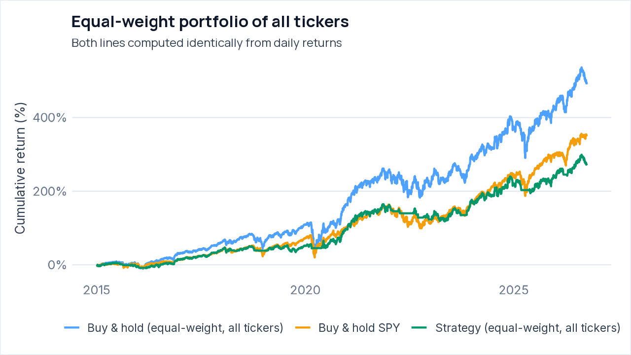
The market-trend filter, which held each stock only while SPY was above its 100-day moving average, beat buy-and-hold by CAGR on 306 of 989 tickers, or 30.9%, during 2015-01-01 to 2026-09-30. The typical result was worse than buy-and-hold, with median excess CAGR of -2.68 percentage points. In the equal-weight portfolio, the strategy had an 11.80% CAGR versus 16.33% for buy-and-hold, while its maximum drawdown was 23.13 percentage points smaller and its Sharpe ratio was higher by 0.05.The main caveat is that the tickers were current S&P 500, S&P 400, and S&P 600 constituents, so companies removed from those indexes during the window are absent, creating survivorship bias. Also, the 989 tickers were not independent: their mean pairwise return correlation was 0.29, and the portfolio excess-return interval ran from -12.42 to 2.67 percentage points, which includes zero.
How Many Tickers Did It Beat Buy-and-Hold On?
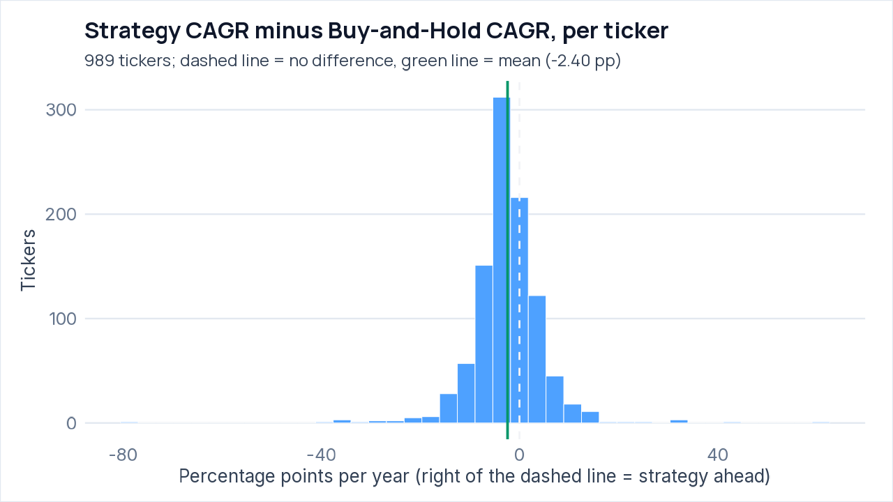
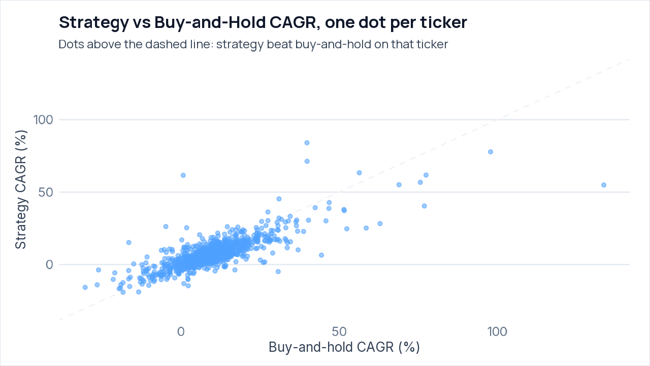
The strategy beat buy-and-hold on an annualized growth rate (CAGR) basis for 306 of 989 tickers, or 30.9%. The excess CAGR versus buy-and-hold had a mean of -2.40 percentage points, a median of -2.68 percentage points, a 10th percentile of -9.15 percentage points, and a 90th percentile of 4.37 percentage points. This means the strategy lagged on most tickers, although the gap was positive for some.
The strategy had a smaller maximum drawdown, the largest decline from a previous peak, on 81.5% of tickers. Median maximum drawdown was 51.83% for the strategy versus 62.86% for buy-and-hold. Its Sharpe ratio, a return measure adjusted for volatility, was better on 32.2% of tickers, with median values of 0.39 versus 0.45, and median time in the market was 79.1%.
Results were consistent in the broad share of winners across the two sub-periods: the strategy beat buy-and-hold on 33.7% of tickers in the first half and 33.5% in the second half. Median excess CAGR remained negative in both, at -22.83 percentage points and -18.64 percentage points. By sector, Communication Services had the highest beat share at 48.5%, followed by Real Estate at 45.3% and Consumer Discretionary at 41.2%; Utilities stood out on the low end at 2.7%, while every sector listed had a negative median excess CAGR.
Is the Result Statistically Significant?
The naive tests point in one direction. The strategy beat buy-and-hold on 306 of 989 tickers, or 30.9%, which is below a 50% coin flip; the exact binomial test gave a p-value of less than 0.0001. A p-value is the probability of seeing a result at least this extreme if there were no real edge. The mean excess CAGR was -2.40 percentage points, with a bootstrap 95% interval of -2.86 to -1.93 percentage points, and the t-test gave t = -10.14 with p = less than 0.0001. On their own, these tests suggest the strategy underperformed buy-and-hold.
Those tests treat the tickers as more independent than they really are. Their mean pairwise correlation was 0.29, making the 989 tickers behave like about 3.5 independent observations; after adjusting for this dependence, the t-statistic was -0.60 and the p-value was 0.5999. That adjusted result is NOT strong evidence of an edge. The equal-weight portfolio comparison also showed lower performance for the strategy, with a CAGR of 11.80% versus 16.33% for buy-and-hold, while the block-bootstrap 95% interval for annualised excess return was -12.42 to 2.67 percentage points, which includes zero and is therefore NOT strong evidence of an edge.
Ticker-level tests found 77 significant tickers at the 5% level, including 76 with a positive mean, while chance alone would produce about 48.6. After the Benjamini-Hochberg false-discovery correction, 0 remained significant, including 0 positive. The pooled-trade test found 50,759 closed trades, a mean return per trade of 2.61%, and p = less than 0.0001, with a 95% interval of 2.42% to 2.80%, but trades overlap in time across tickers, so that p-value is indicative only. The data can show that naive tests and pooled trades look positive in places, but after accounting for ticker dependence and multiple testing, it cannot establish a statistically significant edge over buy-and-hold.
The Equal-Weight Portfolio View
Limits of This Test
What Stood Out
- The strategy portfolio had a lower CAGR than buy-and-hold, 11.80% versus 16.33%, but a smaller maximum drawdown, 17.66% versus 40.79%, and a slightly higher Sharpe ratio, 0.89 versus 0.84.
- The unadjusted excess-CAGR tests had p-values less than 0.0001, but ticker correlation reduced the adjusted result to a t-statistic of -0.60 and a p-value of 0.5999.
- 77 tickers were significant at the 5% level before correction, but 0 remained after Benjamini-Hochberg false-discovery correction.
Limitations
- Survivorship bias applies: Tickers are TODAY’s index members. Companies that were delisted, acquired or removed during the window are absent, which biases buy-and-hold and strategy results upward.
- Tickers are correlated, and each ticker is a standalone backtest rather than a tradable portfolio. The portfolio results therefore do not represent one portfolio holding all positions together under a shared capital allocation.
- The evaluation window may cover a single market regime, so results may not generalize to different market conditions.
- Execution assumes a signal at the close and a fill at the next open, with slippage 5 basis points per fill, no commission, and idle cash earning 0%.
- 11 of 1000 requested tickers were excluded: 1 because the lookback was outside the valid range [1, 66], 1 because it was outside [1, 87], 1 because the series contained non-leading missing values, 5 because they had fewer than 504 bars, and 3 because no price data was returned.
Conclusions
This backtest showed lower returns than buy-and-hold in the equal-weight portfolio, with an 11.80% CAGR versus 16.33%, but a smaller maximum drawdown of 17.66% versus 40.79%. The honest verdict is that it may have reduced drawdowns, but it did not establish a reliable edge over buy-and-hold.The biggest caveat is survivorship bias: the test used current index constituents, so companies removed, acquired, or delisted during the window were absent. This is an educational backtest walkthrough, not investment advice, and past performance in a backtest does not predict future results.
Setup, Audit & Replication
View the exact strategy definition (R) ▾
# =========================================================
# trend_regime_family.R  -- PRE-REGISTERED strategy family (written before any
# results were examined).
#
# One rule family, nine variants: be long a stock while a simple moving-average
# trend condition holds, otherwise sit in cash.
#   filter = "own"    : the stock's close is above its own N-day simple moving average
#   filter = "market" : the market's (SPY) close is above SPY's own N-day moving average
#   filter = "both"   : both conditions hold
#   lookback N in {100, 150, 200} trading days
# Entry when the condition becomes true, exit when it becomes false. Signals are
# evaluated at each bar's close and filled at the next open (engine rule).
# The only free choices are `filter` and `lookback`; they are picked on a
# training set of tickers and an earlier period, then frozen and tested on
# different tickers and a later period (see research_trend_regime.R).
# =========================================================

trend_regime_signals <- function(ohlc, params, market_close) {
  cl <- as.numeric(quantmod::Cl(ohlc))
  n  <- params$lookback
  own_ok    <- cl > TTR::SMA(cl, n)
  market_ok <- market_close > TTR::SMA(market_close, n)
  cond <- switch(params$filter, own = own_ok, market = market_ok, both = own_ok & market_ok)
  list(entry = cond %in% TRUE, exit = (!cond) %in% TRUE)   # NA (insufficient history) -> no action
}

trend_regime_description <- function(filter, lookback) {
  what <- switch(filter,
    own    = sprintf("the stock's closing price is above its own %d-day simple moving average", lookback),
    market = sprintf("the S&P 500 index fund (SPY) closes above its own %d-day simple moving average", lookback),
    both   = sprintf("both the stock's closing price is above its own %d-day simple moving average and SPY closes above its own %d-day simple moving average", lookback, lookback))
  sprintf("Hold the stock (100%% of the capital allotted to it, no leverage) while %s; otherwise hold cash. The condition is checked at each day's close and acted on at the next day's open.", what)
}

make_variant_spec <- function(filter, lookback) {
  list(name = sprintf("Trend filter (%s, %d-day)", filter, lookback),
       description = trend_regime_description(filter, lookback),
       params = list(filter = filter, lookback = lookback),
       needs_market = TRUE,
       signals = trend_regime_signals)
}

trend_regime_variants <- function() {
  g <- expand.grid(filter = c("own", "market", "both"), lookback = c(100, 150, 200), stringsAsFactors = FALSE)
  lapply(seq_len(nrow(g)), function(i) list(id = sprintf("%s_%d", g$filter[i], g$lookback[i]), filter = g$filter[i], lookback = g$lookback[i],
                                            label = sprintf("%s filter, %d-day", c(own = "Own-trend", market = "Market-trend", both = "Own + market trend")[[g$filter[i]]], g$lookback[i])))
}

# FROZEN after selection on training data (see selection.json): filter = "market", lookback = 100
strategy_spec <- make_variant_spec("market", 100)
Integrity Audit: 6 of 6 checks passed
- ✅ Strategy Signals Use Only Past Data: Signals recomputed on truncated history matched the full-history signals at 6 test points.
- ✅ Sample Is Large Enough for Cross-Ticker Statistics: 989 usable tickers (minimum 100)
- ✅ Few Tickers Excluded: 11 of 1000 requested tickers excluded
- ✅ No Ticker Has Missing Headline Metrics: 989 tickers checked
- ✅ Buy-and-Hold Returns Recomputed From Raw Prices Match: REXR: 224.05% vs recorded 224.05% | AXTA: 24.61% vs recorded 24.61% | SONO: 11.51% vs recorded 11.51% | TRST: 136.09% vs recorded 136.09%
- ✅ Independent Cash-Accounting Re-Simulation Matches the Engine: REXR: 215.90% vs recorded 215.90% | AXTA: -14.88% vs recorded -14.88% | SONO: 109.44% vs recorded 109.44% | TRST: 77.85% vs recorded 77.85%