Summary
This article implements the rule in Section 4.1 of Kakushadze & Serur (2018), 151 Trading Strategies: each month, rank sector ETFs by their return over the past year and hold the leaders. We apply it to the nine original SPDR sector funds (technology, energy, health care and so on) from January 2000 to October 2026.
Holding the top three funds returned 8.69% a year, about the same as holding all nine equally (8.92%, charged the same trading costs) and the S&P 500 (8.17%), but with a smaller worst fall from a peak: −39.2% against −49.2% and −50.8%. Holding only the top one, the closest we can get to the paper’s “top decile” with nine funds, returned less (7.17%) and fell as far as the others (−49.2%). The edge is not robust: the top-three portfolio beat equal weighting in 10 of 27 calendar years, and only 2 of 16 parameter settings beat its Sharpe ratio.
Introduction
Momentum is one of the best-documented patterns in investing: assets that have done well recently tend to keep doing well for a few more months. This strategy applies that idea to sectors. The U.S. stock market can be split into sectors, and each one can be bought through a sector ETF, a fund that trades like a share. We use the nine original SPDR sector funds: XLB materials, XLE energy, XLF financials, XLI industrials, XLK technology, XLP consumer staples, XLU utilities, XLV health care and XLY consumer discretionary.
The rule: on the last trading day of each month, rank the funds by their return over the previous 12 months, buy the best ones in equal parts and hold them for a month. Then repeat. We hold the portfolio fully invested, long only. The question is whether rotating into the leaders beats holding all nine sectors in equal parts, which is the same stocks without any rotation, and beats SPY, the S&P 500 fund.
Data and methodology
What the paper specifies and what we chose
The paper gives a formula and typical ranges, not a fully specified backtest and not results. This is therefore one explicit implementation of the strategy, not a reproduction of published returns.
| Element | Paper, §4.1 | This article |
|---|---|---|
| Signal | Cumulative return over T months, Eq. (361) | Same, T = 12 |
| Formation period | Typically 6 to 12 months | 12 months |
| Holding period | Typically 1 to 3 months | 1 month |
| Universe | Sector or industry ETFs, none specified | The nine original Select Sector SPDRs, all trading since Dec 1998 |
| Selection | For example the top decile, optionally shorting the bottom decile | Top 1 of 9 (11%, the closest to a decile) and top 3 of 9 (33%, diversified). Long only |
| Weights | Not specified | Equal weights |
| Trading costs | Not specified | 10 bps per unit traded, on drift-adjusted turnover |
| Execution | “Right after time t” | Idealised: at the month-end close that produced the signal |
| Not implemented | MA filter (§4.1.1), dual momentum (§4.1.2) | Separate articles. Also no short leg |
Data. Daily closing prices from Yahoo Finance, adjusted for dividends and splits, for the nine ETFs and SPY, from December 1998 to October 2026, converted to month-end prices. The first 12 months are needed for the first signal, so every result starts in January 2000 and covers 322 months. All strategies, benchmarks and sensitivity tests use exactly these months. Every rotation variant starts with fresh capital at the December 1999 signal and pays one full initial purchase cost; earlier prices are used only to form signals. We use the original nine funds because all have existed since 1998. The eleven funds that exist today add real estate (2015) and communication services (2018), which would shorten the history. The settings were chosen by us from the paper’s ranges before running anything, but not independently registered, so we report all 16 variants below.
The paper writes the denominator of Eq. (361) as Pi(t+T) and notes that t+T is T months in the past. We write t−T with time running forward. It is the same quantity. Equations labelled A1 to A4 are our formalisation of the paper’s verbal description.
Eq. (361): measure momentum
Pi(t) is the adjusted closing price of ETF i at the end of month t and T = 12. Ri(t) is the ETF’s return over the window: 0.20 means +20%.
One number per ETF: how much it has gained or lost over the past year. This is the only information the strategy uses.
sect = px_m[SECTORS]
rcum = sect / sect.shift(T) - 1 # Eq. (361), known at end of month mrcum <- P[m, ] / P[m - T, ] - 1 # Eq. (361)A1: select the winners
Rank 1 is the highest Ri(t). S(t) is the set of the top N ETFs.
This is the paper’s “buy the top decile”. Only the order matters, not the size of the gains, so even in a crash the strategy holds the least-bad sectors rather than going to cash. With nine ETFs a decile is less than one fund, so we run N = 1 and N = 3.
rank = rcum.rank(axis=1, ascending=False, method="first")
w_signal = (rank <= n).astype(float).where(rcum.notna())top <- order(rcum, decreasing = TRUE)[1:n]A2: weight them equally
With N = 3, each selected ETF gets one third of the portfolio and the other six get nothing.
The weights add up to 1, so there is no cash and no shorting. N sets how concentrated the bet is: N = 1 is all-in on one sector, and N = 9 is the equal-weight benchmark with no rotation. We use that case as the benchmark, so it runs through exactly the same code and cost model.
w_signal = w_signal.div(w_signal.sum(axis=1), axis=0) # equal weightw <- rep(0, length(SECTORS)); w[top] <- 1 / nA3 and A4: earn next month’s return, pay costs
ri(t+1) is the ETF’s return over the following month and c = 0.10%. di(t) is last month’s weight after the price moves.
The first term of A3 is the weighted return of the chosen ETFs. The t+1 means we trade at the close of month t and earn month t+1, so a signal never uses the period it is paid on; in the code this is shift(1), and removing it would look into the future. This assumes we can trade at the same close that produced the signal, an idealised close-to-close backtest.
The second term is the trading cost. Weights drift during the month because ETFs move by different amounts, so even keeping the same holdings means trading back to equal weights. A4 gives the drifted weights, and cost is charged on the distance from them to the new targets. For example, from January to February 2009 the same three ETFs stayed on top, yet restoring equal weights took trades worth 2.2% of the portfolio. Counting only changes in the target would show zero.
r = sect.pct_change()                       # month-m return of each ETF
w = w_signal.shift(1)                       # trade at month-end, earn NEXT month
gross = (w * r).sum(axis=1, min_count=1)
drifted = w * (1 + r)                       # last month's weights after the month's price moves
drifted = drifted.div(drifted.sum(axis=1), axis=0)
turnover = (w - drifted.shift(1)).abs().sum(axis=1)   # trades needed to get back to target
net = gross - turnover * cost_bps / 1e4g <- sum(w * r[m + 1, ]) # earned over NEXT month
drifted <- w_prev * (1 + r[m, ]) # last month's weights after the month's price moves
drifted <- drifted / sum(drifted)
tn <- if (m == first_signal) 1 else sum(abs(w - drifted)) # trades needed; first month buys everything
net[m + 1] <- g - tn * cost_bps / 1e4Checks. We wrote the strategy twice, in Python (vectorised pandas) and in R (a month-by-month loop). Each downloads its own prices. All 322 monthly returns of every series agree to within 5e-11, and the results table and all 16 sensitivity results match. We also recomputed two cases by hand from raw prices with plain loops: the December 2008 signal (top three XLP, XLV and XLU, January 2009 return of −2.8610%, identical to the backtest), and the February 2009 turnover above.
Results
| Top 3 of 9 | Top 1 of 9 | Equal-weight 9 | SPY | |
|---|---|---|---|---|
| $100 invested in Jan 2000 became | $937 | $641 | $989 | $823 |
| CAGR | 8.69% | 7.17% | 8.92% | 8.17% |
| Annual volatility | 14.75% | 20.65% | 14.71% | 15.11% |
| Sharpe ratio (risk-free = 0) | 0.64 | 0.44 | 0.66 | 0.60 |
| Maximum drawdown | −39.2% | −49.2% | −49.2% | −50.8% |
| Months with a gain | 61.2% | 57.5% | 65.2% | 63.0% |
| Average monthly turnover | 46% | 64% | 3% | 0% |
January 2000 to October 2026. Both strategies and the equal-weight portfolio are net of the same 10 bps cost model; the equal-weight portfolio is rebalanced monthly. SPY is buy-and-hold with no trading costs. CAGR is the compound annual growth rate, the Sharpe ratio is return per unit of volatility, and maximum drawdown is the largest fall from a previous peak. Before costs the top-three portfolio earned 9.29% a year (Sharpe 0.68). Its 46% monthly turnover costs 0.55 percentage points a year (turnover × cost × 12); the gap between gross and net CAGR is 0.60, which includes compounding.
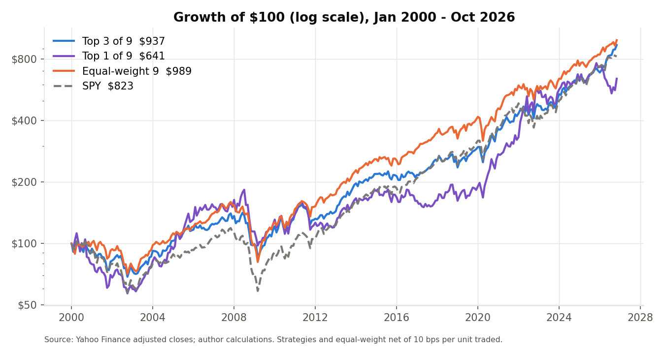
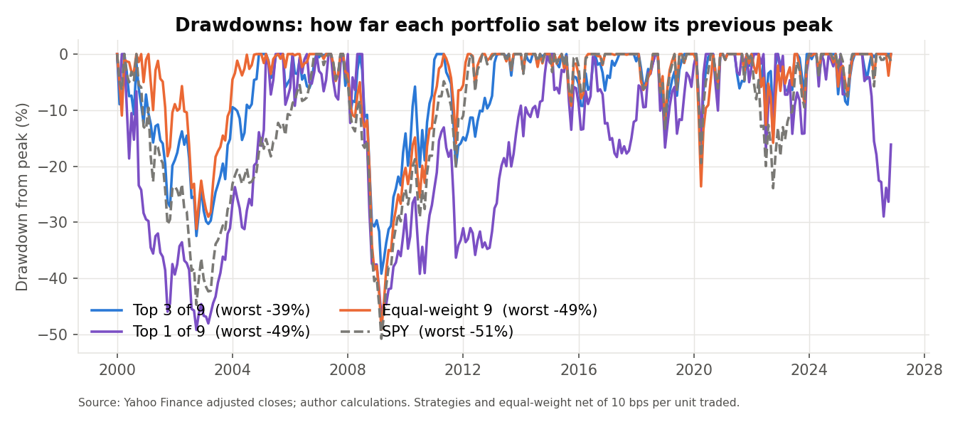
Concentration did not pay: the top-one portfolio returned 7.17% with 20.6% volatility (against 14.8% for top three), and a 64% monthly turnover. It had one spectacular year, 64% in 2022, when energy led, and long stretches of lagging. The top-three portfolio did not beat equal weighting on return and won in only 10 of 27 calendar-year observations (2026 is January to October). A retrospective split shows it trailed equal weighting from 2000 to 2012 (2.8% against 4.4% a year) and led from 2013 to 2026 (14.5% against 13.4%). The dates were chosen after seeing the results, so this is context, not out-of-sample evidence.
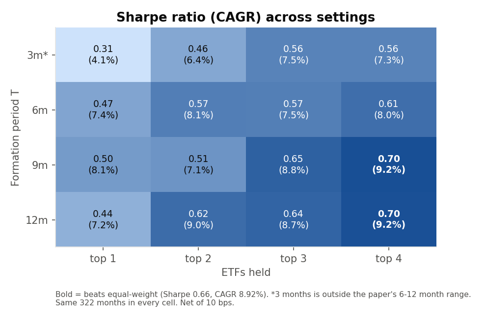
To test whether the settings were lucky, we re-ran 16 combinations of T ∈ {3, 6, 9, 12} months and N ∈ {1, 2, 3, 4} ETFs on the same 322 months. These are an exploration of sensitivity, not 16 confirmations of the paper’s strategy, and 3 months lies outside the paper’s 6 to 12 month range. Sharpe ratios range from 0.31 to 0.70. Only 2 settings beat the equal-weight portfolio’s 0.66: the 9-month look-back with 4 ETFs and 12-month look-back with 4 ETFs. The weakest setting earns 4.1% a year.
Conclusion
Under the implementation choices used in this study, sector momentum rotation did not outperform an equally weighted portfolio of the nine original SPDR sector ETFs on CAGR or Sharpe ratio. The strategy follows the momentum-ranking framework in Kakushadze and Serur (2018), while the universe, portfolio concentration, weighting method and transaction-cost assumptions are specified independently. In this sample, the top-three portfolio had a smaller maximum drawdown but slightly lower return than equal weighting; the top-one portfolio earned less and did not provide comparable drawdown protection. Across 16 settings the evidence for an edge is weak. These observations do not establish a general benefit from diversification in sector momentum.
Limitations. Nine ETFs is a small universe and cannot express a true decile, nor the eleven sectors that exist today. Execution is idealised: trades happen at the same close that produced the signal. Costs are a flat 10 bps; taxes, wider spreads and market impact are ignored. The strategy is long only, without the paper’s optional short leg. Yahoo can revise adjusted prices, so rerunning the code later may give slightly different numbers. Past results are not a forecast. The moving-average filter (§4.1.1) and dual momentum (§4.1.2) are covered in separate articles.
Code
Each script is self-contained: it downloads the prices, runs the strategy, prints the results table and draws the three charts shown above. Copy it into a file and run it. Nothing is written to disk. The shaded block is the strategy function, the code behind Eq. (361) and A1 to A4. The results above were produced with Python 3.13.2, pandas 2.3.3, numpy 2.5.3, yfinance 0.2.64; R 4.5.0, quantmod 0.4.28, xts 0.14.1. The scripts also accept an archived adjusted-price CSV through the QST_PRICE_SNAPSHOT environment variable. A fixed sample alone does not freeze Yahoo prices. The local review package preserves the exact adjusted prices, scripts, monthly returns, weights, package versions and SHA-256 checksums used for these figures. Publication of that package is subject to reviewer approval and data-redistribution permission; we do not claim the price snapshot is already public. The previously released monthly returns and weights are in the GitHub repository.
"""4.1 Strategy: Sector momentum rotation -- implementation of Kakushadze & Serur (2018),
"151 Trading Strategies", Section 4.1, Eq. (361).

    R_cum_i(t) = P_i(t) / P_i(t - T) - 1      (T months back from t)

At each month-end t: rank the sector ETFs by R_cum_i(t), buy the top N equal-weighted,
hold for one month (the paper's 1-3 month holding period), then repeat.
N = 1 is the closest to the paper's "top decile" with nine ETFs; N = 3 is a diversified version.
N = 9 holds every ETF equally, which is the no-rotation benchmark.
"""
import os
import numpy as np
import pandas as pd
import matplotlib.pyplot as plt
import yfinance as yf   # pip install yfinance

SECTORS = ["XLB", "XLE", "XLF", "XLI", "XLK", "XLP", "XLU", "XLV", "XLY"]
T_MONTHS = 12      # formation period (paper: 6-12 months)
TOP_N = 3          # diversified version; N = 1 is the closest to the paper's top decile
COST_BPS = 10      # cost per unit of turnover, in basis points
# Fixed historical sample; Yahoo data may be revised
START, END = "1998-12-01", "2026-11-01"
FIRST_RETURN = "2000-01-31"  # all variants start with fresh capital; signal is Dec 1999


def download_prices():
    """Daily adjusted closes for the 9 sector ETFs + SPY, straight from Yahoo Finance."""
    snapshot = os.getenv("QST_PRICE_SNAPSHOT")
    if snapshot:
        return pd.read_csv(snapshot, index_col=0, parse_dates=True)[SECTORS + ["SPY"]]
    tickers = SECTORS + ["SPY"]
    px = yf.download(tickers, start=START, end=END, auto_adjust=True, progress=False)["Close"]
    return px[tickers].dropna(how="all")


def to_monthly(px):
    return px.resample("ME").last()             # last trading day of each month


def run(px_m, T=T_MONTHS, n=TOP_N, cost_bps=COST_BPS, start=FIRST_RETURN):
    sect = px_m[SECTORS]
    r = sect.pct_change()                       # month-m return of each ETF
    rcum = sect / sect.shift(T) - 1             # Eq. (361), known at end of month m
    rank = rcum.rank(axis=1, ascending=False, method="first")
    w_signal = (rank <= n).astype(float).where(rcum.notna())
    w_signal = w_signal.div(w_signal.sum(axis=1), axis=0)   # equal weight
    w = w_signal.shift(1)                       # trade at month-end, earn NEXT month
    w = w.loc[pd.Timestamp(start):].copy()        # warm-up prices inform signals, never prior holdings
    if w.empty or w.iloc[0].isna().any():
        raise ValueError("Insufficient history at the common fresh-capital start")
    r = r.loc[w.index]
    gross = (w * r).sum(axis=1, min_count=1)
    drifted = w * (1 + r)                       # last month's weights after the month's price moves
    drifted = drifted.div(drifted.sum(axis=1), axis=0)
    turnover = (w - drifted.shift(1)).abs().sum(axis=1)   # trades needed to get back to target
    first = w.dropna(how="all").index[0]
    turnover.loc[first] = 1.0                   # initial purchase
    net = gross - turnover * cost_bps / 1e4
    out = pd.DataFrame({"gross": gross, "net": net, "turnover": turnover}).loc[first:]
    return out, w.loc[first:], rcum


def stats(ret, label=""):
    ret = ret.dropna()
    yrs = len(ret) / 12
    eq = np.r_[1.0, (1 + ret).cumprod().to_numpy()]      # starts at 1 so an initial loss counts
    dd = eq / np.maximum.accumulate(eq) - 1
    return {
        "label": label,
        "start": str(ret.index[0].date()), "end": str(ret.index[-1].date()),
        "months": int(len(ret)),
        "total_return_pct": round(float(eq[-1] - 1) * 100, 2),
        "cagr_pct": round(float(eq[-1] ** (1 / yrs) - 1) * 100, 2),
        "ann_vol_pct": round(float(ret.std(ddof=1) * np.sqrt(12)) * 100, 2),
        "sharpe": round(float(ret.mean() / ret.std(ddof=1) * np.sqrt(12)), 3),
        "max_drawdown_pct": round(float(dd.min()) * 100, 2),
        "hit_rate_pct": round(float((ret > 0).mean()) * 100, 1),
    }


def results_table(summary):
    """Net-of-cost results side by side, as a DataFrame."""
    cols = {"Top 3 of 9": "top3", "Top 1 of 9": "top1", "Equal-weight 9 (net)": "equal_weight", "SPY": "spy"}
    return pd.DataFrame({name: {
        "$100 became": 100 * (1 + summary[k]["total_return_pct"] / 100),
        "CAGR (%)": summary[k]["cagr_pct"], "Volatility (%)": summary[k]["ann_vol_pct"],
        "Sharpe": summary[k]["sharpe"], "Max drawdown (%)": summary[k]["max_drawdown_pct"],
        "Months with a gain (%)": summary[k]["hit_rate_pct"],
        "Monthly turnover (%)": summary["avg_monthly_turnover_pct"].get(k, 0.0)}
        for name, k in cols.items()})


def plot_results(top3, top1, ew, spy, grid):
    eq = 100 * (1 + pd.DataFrame({"Top 3 of 9": top3, "Top 1 of 9": top1,
                                  "Equal-weight 9 (net)": ew, "SPY": spy})).cumprod()
    colors, styles = ["#2a78d6", "#7b4fc4", "#eb6834", "grey"], ["-", "-", "-", "--"]
    fig, ax = plt.subplots(3, 1, figsize=(9, 12))
    for c, col, ls in zip(eq.columns, colors, styles):
        ax[0].plot(eq.index, eq[c], color=col, ls=ls, lw=2, label=c)
        ax[1].plot(eq.index, 100 * (eq[c] / eq[c].cummax().clip(lower=100) - 1), color=col, ls=ls, lw=2)
    ax[0].set_yscale("log"); ax[0].set_title("Growth of $100 (log scale)"); ax[0].legend(frameon=False)
    ax[1].set_title("Drawdown from previous peak (%)")
    Ts, Ns = (3, 6, 9, 12), (1, 2, 3, 4)
    sharpe = np.array([[grid[f"T{T}_N{n}"]["sharpe"] for n in Ns] for T in Ts])
    ax[2].imshow(sharpe, cmap="Blues")
    ax[2].set_xticks(range(4), Ns); ax[2].set_yticks(range(4), Ts)
    ax[2].set_xlabel("ETFs held (n)"); ax[2].set_ylabel("Look-back T (months)")
    ax[2].set_title("Sharpe ratio by setting (same sample for every cell)")
    for i in range(4):
        for j in range(4):
            ax[2].text(j, i, f"{sharpe[i, j]:.2f}", ha="center", va="center")
    fig.tight_layout()
    plt.show()


def main():
    px = download_prices()
    px_m = to_monthly(px)
    top3, w, rcum = run(px_m)                   # top 3 of 9
    top1 = run(px_m, n=1)[0]                    # top 1 of 9: closest to the paper's top decile
    ew = run(px_m, n=9)[0]                      # all 9 equally, rebalanced monthly, same costs
    idx = top3.index                            # one common sample for everything
    spy = px_m["SPY"].pct_change().loc[idx]

    summary = {
        "params": {"T_months": T_MONTHS, "top_n": TOP_N, "cost_bps": COST_BPS, "first_return": FIRST_RETURN, "universe": SECTORS},
        "top3": stats(top3["net"], "Top 3 of 9 (net)"),
        "top3_gross": stats(top3["gross"], "Top 3 of 9 (gross)"),
        "top1": stats(top1["net"], "Top 1 of 9 (net)"),
        "equal_weight": stats(ew["net"], "Equal-weight 9 (net)"),
        "equal_weight_gross": stats(ew["gross"], "Equal-weight 9 (gross)"),
        "spy": stats(spy, "SPY buy & hold"),
        "avg_monthly_turnover_pct": {"top3": round(float(top3["turnover"].mean()) * 100, 1),
                                     "top1": round(float(top1["turnover"].mean()) * 100, 1),
                                     "equal_weight": round(float(ew["turnover"].mean()) * 100, 1)},
    }
    # sensitivity grid: every cell is evaluated on the same months as the main result
    grid = {}
    for T in (3, 6, 9, 12):
        for n in (1, 2, 3, 4):
            s = stats(run(px_m, T, n)[0]["net"].reindex(idx))
            grid[f"T{T}_N{n}"] = {"cagr_pct": s["cagr_pct"], "sharpe": s["sharpe"],
                                    "start": s["start"], "end": s["end"], "months": s["months"],
                                    "initial_turnover": float(run(px_m, T, n)[0]["turnover"].iloc[0])}
    summary["sensitivity"] = grid
    # calendar-year returns
    yr = pd.DataFrame({"top3": top3["net"], "top1": top1["net"], "equal_weight": ew["net"], "spy": spy})
    summary["annual_returns_pct"] = (
        ((1 + yr).groupby(yr.index.year).prod() - 1) * 100).round(2).to_dict("index")

    # ---- SAVE-BEGIN: optional, uncomment to write the results to ./data ----
    # import json
    # from pathlib import Path
    # out = Path("data"); out.mkdir(exist_ok=True)
    # px.to_csv(out / "prices_python.csv")
    # (out / "results_python.json").write_text(json.dumps(summary, indent=2, default=str))
    # pd.DataFrame({"top3_net": top3["net"], "top3_gross": top3["gross"], "top1_net": top1["net"],
    #               "ew_net": ew["net"], "ew_gross": ew["gross"], "spy": spy, "turnover_top3": top3["turnover"]}
    #              ).to_csv(out / "monthly_returns_python.csv", float_format="%.10f")
    # w.to_csv(out / "weights_python.csv", float_format="%.6f")
    # ---- SAVE-END ----

    print(results_table(summary).round(2).to_string())
    plot_results(top3["net"], top1["net"], ew["net"], spy, grid)
    return top3, w, rcum, px_m, ew, spy, summary


if __name__ == "__main__":
    main()
# 4.1 Strategy: Sector momentum rotation -- implementation of Kakushadze & Serur (2018),
# "151 Trading Strategies", Section 4.1, Eq. (361):
#     R_cum_i(t) = P_i(t) / P_i(t - T) - 1      (T months back from t)
# Each month-end: rank sector ETFs by R_cum, buy the top N equal-weighted, hold 1 month.
# N = 1 is the closest to the paper's "top decile" with nine ETFs; N = 3 is a diversified version.
# N = 9 holds every ETF equally, which is the no-rotation benchmark.
suppressPackageStartupMessages({ library(quantmod); library(xts) })
# install.packages(c("quantmod", "xts"))   # once

SECTORS <- c("XLB","XLE","XLF","XLI","XLK","XLP","XLU","XLV","XLY")
T_MONTHS <- 12; TOP_N <- 3; COST_BPS <- 10
# Fixed historical sample; Yahoo data may be revised
START <- "1998-12-01"; END <- "2026-10-31"
FIRST_RETURN <- "2000-01"  # all variants start with fresh capital; signal is Dec 1999

# Daily adjusted closes for the 9 sector ETFs + SPY, straight from Yahoo Finance
TICKERS <- c(SECTORS, "SPY")
snapshot <- Sys.getenv("QST_PRICE_SNAPSHOT")
if (nzchar(snapshot)) {
  archived <- read.csv(snapshot, check.names = FALSE)
  px <- xts(as.matrix(archived[, TICKERS]), order.by = as.Date(archived[[1]]))
} else {
  px <- do.call(merge, lapply(TICKERS, function(s)
    Ad(getSymbols(s, src = "yahoo", from = START, to = END, auto.assign = FALSE))))
}
colnames(px) <- TICKERS
pm <- apply.monthly(px, function(x) tail(x, 1))        # month-end prices
index(pm) <- as.Date(format(index(pm), "%Y-%m-01")) # label by month
months <- format(index(pm), "%Y-%m")

run_strategy <- function(pm, T = T_MONTHS, n = TOP_N, cost_bps = COST_BPS, start = FIRST_RETURN) {
  P <- coredata(pm[, SECTORS]); N <- nrow(P)
  r <- rbind(NA, P[-1, ] / P[-N, ] - 1)                # monthly returns
  w_prev <- rep(0, length(SECTORS))                    # weights held during month m
  gross <- net <- turn <- rep(NA_real_, N)
  first_signal <- match(start, format(index(pm), "%Y-%m")) - 1L
  if (is.na(first_signal) || first_signal < T + 1L || first_signal >= N) stop("Insufficient history at common start")
  for (m in first_signal:(N - 1)) {                         # signal at end of month m
    rcum <- P[m, ] / P[m - T, ] - 1                    # Eq. (361)
    top <- order(rcum, decreasing = TRUE)[1:n]
    w <- rep(0, length(SECTORS)); w[top] <- 1 / n
    g <- sum(w * r[m + 1, ])                           # earned over NEXT month
    drifted <- w_prev * (1 + r[m, ])                   # last month's weights after the month's price moves
    drifted <- drifted / sum(drifted)
    tn <- if (m == first_signal) 1 else sum(abs(w - drifted)) # trades needed; first month buys everything
    gross[m + 1] <- g
    net[m + 1] <- g - tn * cost_bps / 1e4
    turn[m + 1] <- tn
    w_prev <- w
  }
  data.frame(month = months, gross = gross, net = net, turnover = turn)
}

stats <- function(ret, label) {
  ret <- ret[!is.na(ret)]; yrs <- length(ret) / 12
  eq <- c(1, cumprod(1 + ret)); dd <- eq / cummax(eq) - 1   # starts at 1 so an initial loss counts
  list(label = label, months = length(ret),
       total_return_pct = round((tail(eq, 1) - 1) * 100, 2),
       cagr_pct = round((tail(eq, 1)^(1 / yrs) - 1) * 100, 2),
       ann_vol_pct = round(sd(ret) * sqrt(12) * 100, 2),
       sharpe = round(mean(ret) / sd(ret) * sqrt(12), 3),
       max_drawdown_pct = round(min(dd) * 100, 2),
       hit_rate_pct = round(mean(ret > 0) * 100, 1))
}

top3 <- run_strategy(pm)                       # top 3 of 9
top1 <- run_strategy(pm, n = 1)                # top 1 of 9: closest to the paper's top decile
ew   <- run_strategy(pm, n = 9)                # all 9 equally, rebalanced monthly, same costs
ok <- !is.na(top3$net)                         # one common sample for everything
spy <- c(NA, as.numeric(pm[-1, "SPY"]) / as.numeric(pm[-nrow(pm), "SPY"]) - 1)

# ---- Results table (net of costs) ----
rows <- c("total_return_pct", "cagr_pct", "ann_vol_pct", "sharpe", "max_drawdown_pct", "hit_rate_pct")
col <- function(x, turnover) { s <- stats(x[ok], ""); c(100 * (1 + s$total_return_pct / 100), unlist(s[rows[-1]]), turnover) }
results <- data.frame(
  Metric = c("$100 became", "CAGR (%)", "Volatility (%)", "Sharpe", "Max drawdown (%)", "Months with a gain (%)",
             "Monthly turnover (%)"),
  "Top 3 of 9" = col(top3$net, mean(top3$turnover[ok]) * 100), "Top 1 of 9" = col(top1$net, mean(top1$turnover[ok]) * 100),
  "Equal-weight 9 (net)" = col(ew$net, mean(ew$turnover[ok]) * 100), SPY = col(spy, 0),
  check.names = FALSE, row.names = NULL)
results[, -1] <- round(results[, -1], 2)
print(results, row.names = FALSE)

# ---- Sensitivity: every combination of look-back T and number of ETFs held n, on the same months ----
sens <- expand.grid(T_months = c(3, 6, 9, 12), n = 1:4)
sens[c("cagr_pct", "sharpe")] <- t(mapply(function(T, n) {
  trial <- run_strategy(pm, T, n)
  stopifnot(trial$turnover[which(ok)[1]] == 1)
  s <- stats(trial$net[ok], ""); c(s$cagr_pct, s$sharpe) }, sens$T_months, sens$n))
print(sens, row.names = FALSE)

# ---- Plots ----
yr <- as.numeric(format(index(pm)[ok], "%Y")) + (as.numeric(format(index(pm)[ok], "%m")) - 1) / 12
eq <- 100 * cbind("Top 3 of 9" = cumprod(1 + top3$net[ok]), "Top 1 of 9" = cumprod(1 + top1$net[ok]),
                  "Equal-weight 9 (net)" = cumprod(1 + ew$net[ok]), SPY = cumprod(1 + spy[ok]))
cols <- c("#2a78d6", "#7b4fc4", "#eb6834", "grey40"); ltys <- c(1, 1, 1, 2)
par(mfrow = c(3, 1), mar = c(3, 4, 3, 1))
matplot(yr, eq, type = "l", col = cols, lty = ltys, lwd = 2, log = "y", xlab = "", ylab = "$",
        main = "Growth of $100 (log scale)")
legend("topleft", colnames(eq), col = cols, lty = ltys, lwd = 2, bty = "n")
matplot(yr, 100 * (eq / apply(eq, 2, function(x) pmax(100, cummax(x))) - 1), type = "l", col = cols, lty = ltys, lwd = 2, xlab = "",
        ylab = "%", main = "Drawdown from previous peak")
M <- matrix(sens$sharpe, nrow = 4)           # rows = T (3, 6, 9, 12), columns = n (1 to 4)
image(1:4, 1:4, t(M)[, 4:1], col = hcl.colors(20, "Blues", rev = TRUE), axes = FALSE,
      xlab = "ETFs held (n)", ylab = "Look-back T (months)", main = "Sharpe ratio by setting (same sample)")
axis(1, 1:4, 1:4); axis(2, 1:4, rev(c(3, 6, 9, 12)), las = 1)
for (i in 1:4) for (j in 1:4) text(j, 5 - i, sprintf("%.2f", M[i, j]))

# ---- SAVE-BEGIN: optional, uncomment to write the results to ./data ----
# root <- getwd(); dir.create(file.path(root, "data"), showWarnings = FALSE)
# write.csv(data.frame(date = index(px), coredata(px)), file.path(root, "data", "prices_r.csv"), row.names = FALSE)
# write.csv(results, file.path(root, "data", "results_table_r.csv"), row.names = FALSE)
# write.csv(sens, file.path(root, "data", "sensitivity_r.csv"), row.names = FALSE)
# write.csv(data.frame(month = top3$month[ok], top3_net = top3$net[ok], top3_gross = top3$gross[ok],
#           top1_net = top1$net[ok], ew_net = ew$net[ok], ew_gross = ew$gross[ok], spy = spy[ok],
#           turnover_top3 = top3$turnover[ok]),
#           file.path(root, "data", "monthly_returns_r.csv"), row.names = FALSE)
# ---- SAVE-END ----
References
Kakushadze, Z. and Serur, J. A. (2018). 151 Trading Strategies. Available at SSRN: https://ssrn.com/abstract=3247865. Source paper
Implemented here: Chapter 4 (Exchange-traded funds), §4.1 “Strategy: Sector momentum rotation”, Eq. (361), pp. 61–62.
Moskowitz, T. J. and Grinblatt, M. (1999). Do industries explain momentum? The Journal of Finance, 54(4), 1249–1290. doi:10.1111/0022-1082.00146 Cited in the paper
Educational content, not investment advice. Backtested results are not a forecast of future returns.