Summary
This article implements Section 4.3 of Kakushadze & Serur (2018), 151 Trading Strategies. The section proposes ranking funds by the R-squared of a four-factor regression: a fund whose returns are mostly explained by the market, size, value and momentum factors (high R-squared) is behaving like an index, while a fund with a low R-squared is doing something of its own. The book gives the rule and cites no results. The empirical evidence behind it is Amihud and Goyenko (2013), who studied US equity mutual funds from 1990 to 2007. We follow the design of the working-paper version of their study (the published 2013 version reports its main tests with monthly data, and we have not replicated those) on a later period, 2012 to 2025, using 1,362 US equity mutual funds from Yahoo Finance (18,677 fund-years).
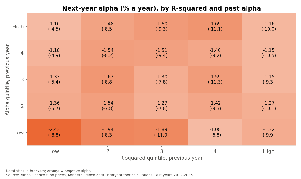
We do not detect the same relationship in this sample. In the original study, the funds with the lowest R-squared and the highest past alpha went on to earn a four-factor alpha of +2.81% a year. Here the same group earned −1.10% a year (t-statistic −4.5), still negative, though above the average fund-year alpha of −1.45%. We find no significant predictive relationship between R-squared and next-year alpha in this sample and specification (coefficient 0.031, t-statistic 0.52; Amihud and Goyenko report −0.680 and 7.69, with fund-characteristic controls that this headline regression lacks). It does still predict the information ratio (alpha divided by residual risk), but that is largely arithmetic when alpha is negative. Year by year, the best group beat the average fund in 7 of 14 calendar years and returned 10.21% a year when funds were chosen once a year, against 12.24% for all funds and 14.86% for SPY. Our monthly long-short adaptation of the book’s rule lost 1.37% a year after costs.
A failure to reproduce is a finding about this period and this data; it does not show that the original result was wrong. The differences between the two samples are listed below.
Introduction
An actively managed fund is meant to differ from the market. A natural way to measure how much it differs is to regress its returns on the standard risk factors and look at the R-squared: the share of the fund’s day-to-day movement that the factors explain. A fund with an R-squared of 0.98 is, for practical purposes, a market fund with a fee attached. A fund with an R-squared of 0.70 is making bets of its own, for better or worse. Section 4.3 of the book turns this into a trading rule: favour funds with a low R-squared (Amihud and Goyenko call this high “selectivity”), and among them those with a high alpha, the part of their return the factors do not explain.
The book describes the rule for exchange-traded funds (ETFs) and gives no data and no results. Its footnote points to Amihud and Goyenko (2013) for the evidence: they found that mutual funds with a low R-squared in one year earned better risk-adjusted returns in the next. Because the book offers nothing to reproduce, we replicate the research it relies on, following the original design and sorting method.
The research we replicate
Amihud and Goyenko studied US equity mutual funds from 1990 to 2007. Their design, as described in their working paper, is:
- One regression per fund-year. For each fund and calendar year, regress daily excess returns on the market, size, value and momentum factors and their one-day lagged values (the lags allow for stocks that react slowly, following Dimson, 1979). Keep the intercept (alpha), the R-squared and the residual standard error (RMSE).
- Predict the next year. The R-squared and alpha of year y−1 are used to predict the alpha and information ratio of year y, the information ratio being alpha divided by RMSE.
- Sort into 25 groups. Each year, funds are sorted into five R-squared groups (quintiles) and, within each, five groups by past alpha. The average next-year alpha of each of the 25 groups is the main result. The exercise is repeated with independent sorts.
- Regressions. Next-year alpha and information ratio are regressed on lagged R-squared, with year and style dummies and standard errors clustered by fund, and with Fama-MacBeth annual cross-sections.
Their headline: the group with the lowest R-squared and highest past alpha earned a four-factor alpha of 2.81% a year (t-statistic 5.84), and the coefficient on transformed R-squared in the alpha regression was −0.680 (t-statistic 7.69). Their sample has about 2,300 funds and 16,600 fund-years. We reproduce these analyses, and we add what the book itself describes, a monthly long-short version, as an extension.
Data and methodology
Differences from the original sample
| Element | Original study | This article |
|---|---|---|
| Fund data | CRSP Survivorship-Bias-Free Mutual Fund Database, plus daily data supplements | Yahoo Finance adjusted closing prices (net of fund expenses, dividends and capital gains reinvested). Yahoo lists live funds only, so this sample is survivorship-biased |
| Period | 1990–2007 test years | 2012–2025 test years (2026, January to September, is reported separately); first estimation year 2011 |
| Funds | Active all-equity funds, index funds removed by name (“index” or “ind”), fund size at least $15 million | US equity funds in Yahoo’s nine style-box categories (large, mid, small; blend, growth, value). Funds with “index” or “ind” in the name removed. No size filter (not available) |
| Share classes | Classes of one fund averaged, weighted by assets | One class per fund (see below) |
| Regression | Daily excess returns on RM−Rf, SMB, HML, momentum and their lags, one calendar year | Same. Factors from Kenneth French’s data library (daily, vintage 202609) |
| Data requirements | At least 125 daily returns in year y−1 and 50 in year y | Same |
| Trimming | Top and bottom 1% of R-squared removed | Same (R-squared kept between 0.44 and 0.99) |
| Transformation | TR² = ln(√R² / (1 − √R²)) | Same |
| Controls | Fund size, expenses, turnover, age, manager tenure, Active Share (year-end values) | Headline results without controls. A separate table uses Yahoo’s current size, expense ratio, turnover and age as proxies. Manager tenure and Active Share are not available |
| Style groups | Four (growth, income, growth and income, small cap) | Yahoo’s nine style-box categories, as dummies |
Building the fund list
Yahoo’s fund screener returned 5,607 US equity funds in the nine style-box categories. Of these, 3,156 had price history starting before mid-2011, so that every test year could have a prior estimation year. Prices from Yahoo are not always clean: 83 funds had at least one daily move beyond ±30% (for example, an unadjusted split recorded as a collapse in price) and were removed. The list is in the repository as a CSV file.
One class per fund. A mutual fund is often sold in several versions, called share classes (A, C, Institutional and so on), with the same portfolio and different fees. Yahoo lists each as a separate ticker, so counting them all would count one fund many times and place near-identical returns in the same sort. We merged tickers whose daily returns over 2012–2026 correlate at 0.999 or more, keeping the class with the longest price history (chosen on data availability only, never on performance). This reduced 3,073 tickers to 1,458 distinct funds; a check afterwards found no remaining pair above that correlation. The original averages classes by assets instead, which needs asset data we do not have. Removing 96 funds with “index” in the name leaves 1,362 funds, 19,059 fund-years before trimming and 18,677 after.
The maths
For fund j and calendar year y, the regression (Eq. 365 of the book, the four-factor model, with the one-day lags that Amihud and Goyenko add) is:
Rj(t) is the fund’s daily return minus the daily risk-free rate. Fk(t) are the four factors: the three Fama-French factors (market, size, value) and Carhart’s momentum factor. βj,k is the fund’s loading on factor k today and γj,k on yesterday’s value (the lags). αj is the fund’s alpha and εj(t) the daily residual.
The R-squared is the share of the variation the factors explain (Eqs. 366 to 369 of the book), and the information ratio divides alpha by the residual standard error, RMSE:
SSres is the sum of squared residuals and SStot the sum of squared deviations of the fund’s excess return from its own average. n is the number of days used and k = 9 the number of estimated coefficients. We quote alpha per year (daily alpha × 252).
R-squared is transformed before it is used in regressions, because R-squared is bunched near 1:
The prediction step is then a regression across fund-years, with alpha measured in year y and every predictor measured in year y−1:
Dy and Ds are year and style dummies. Standard errors are clustered by fund, because the same fund appears in several years. The tests use TR² alone, or its components RMSE and SDR (the standard deviation of the fund’s daily excess return).
Results, 2012–2025
The sample
| Panel A | Mean | Median | Std dev | Min | Max |
|---|---|---|---|---|---|
| R² (prior year) | 0.925 | 0.943 | 0.068 | 0.444 | 0.995 |
| Alpha, prior year (% a year) | −1.26 | −1.14 | 4.76 | −35.42 | 59.54 |
| RMSE, daily (%) | 0.28 | 0.25 | 0.15 | 0.03 | 2.38 |
| SDR, daily (%) | 1.12 | 0.98 | 0.49 | 0.31 | 4.00 |
| Alpha, test year (% a year) | −1.45 | −1.29 | 4.99 | −39.92 | 67.03 |
| InfRatio, test year | −0.0220 | −0.0219 | 0.0656 | −0.2766 | 0.2197 |
| Funds / fund-years | 1,361 / 18,677 | ||||
Variables from the 18,677 fund-year observations after trimming. RMSE and SDR are daily, in percent. Fund size, expenses, turnover, age and manager tenure are not available point-in-time from Yahoo. The mean R-squared is 0.93, higher than the 0.86 (median 0.90) in the original sample: these funds sit closer to the factor model.
The 25 groups: R-squared first, then alpha
Each year, funds are sorted into five R-squared groups using year y−1, and within each group into five alpha groups, again using year y−1. Each cell is the average year-y four-factor alpha, in percent a year, of every fund-year in that group, with the t-statistic in brackets. The original does not say how its t-statistics are computed. Ours treat each fund-year as one observation; observations within one year are correlated, so they are generous. A stricter test uses the 14 annual averages of one group and is given below.
Panel A. Four-factor alpha, next year (% a year)
| Alphay-1 | R²y-1 quintile | All | Low − High | ||||
|---|---|---|---|---|---|---|---|
| Low | 2 | 3 | 4 | High | |||
| Low | −2.433(−8.82) | −1.937(−8.26) | −1.894(−10.99) | −1.084(−6.82) | −1.315(−9.86) | −1.733(−19.13) | −1.118(−3.65) |
| 2 | −1.358(−5.71) | −1.538(−7.82) | −1.267(−7.83) | −1.422(−9.33) | −1.274(−10.09) | −1.372(−17.13) | −0.083(−0.31) |
| 3 | −1.330(−5.37) | −1.669(−8.78) | −1.296(−7.83) | −1.594(−11.29) | −1.146(−9.34) | −1.407(−17.60) | −0.184(−0.67) |
| 4 | −1.182(−4.94) | −1.544(−8.21) | −1.506(−9.45) | −1.400(−9.21) | −1.146(−10.52) | −1.356(−17.33) | −0.036(−0.14) |
| High | −1.101(−4.53) | −1.481(−8.47) | −1.603(−9.28) | −1.695(−11.06) | −1.156(−9.96) | −1.407(−17.78) | 0.055(0.21) |
| All | −1.478(−13.25) | −1.633(−18.47) | −1.513(−20.30) | −1.440(−21.22) | −1.207(−22.19) | −1.454(−39.80) | −0.271(−2.19) |
| High – Low | 1.332(3.62) | 0.457(1.56) | 0.291(1.19) | −0.611(−2.77) | 0.159(0.90) | 0.325(2.70) | |
Panel B. Information ratio, next year (alpha divided by RMSE, daily)
| InfRatioy-1 | R²y-1 quintile | All | Low − High | ||||
|---|---|---|---|---|---|---|---|
| Low | 2 | 3 | 4 | High | |||
| Low | −0.020(−8.24) | −0.024(−9.29) | −0.026(−11.29) | −0.019(−7.66) | −0.029(−11.35) | −0.024(−21.34) | 0.009(2.63) |
| 2 | −0.019(−7.85) | −0.018(−7.50) | −0.015(−6.31) | −0.023(−9.63) | −0.030(−11.67) | −0.021(−19.28) | 0.012(3.29) |
| 3 | −0.020(−7.58) | −0.023(−9.79) | −0.018(−8.23) | −0.025(−11.10) | −0.028(−11.90) | −0.023(−21.59) | 0.009(2.41) |
| 4 | −0.017(−6.95) | −0.018(−7.20) | −0.022(−9.25) | −0.023(−9.82) | −0.030(−12.23) | −0.022(−20.27) | 0.013(3.93) |
| High | −0.012(−5.35) | −0.019(−8.42) | −0.023(−9.37) | −0.027(−11.39) | −0.023(−10.22) | −0.021(−20.06) | 0.012(3.66) |
| All | −0.017(−16.13) | −0.020(−18.83) | −0.021(−19.85) | −0.023(−22.07) | −0.028(−25.66) | −0.022(−45.84) | 0.011(7.08) |
| High – Low | 0.008(2.54) | 0.005(1.53) | 0.004(1.10) | −0.007(−2.16) | 0.006(1.77) | 0.003(2.09) | |
Rows: previous-year alpha (Panel A) or information ratio (Panel B), within each R-squared quintile. “All” is the average of everything in that row or column. “Low − High” is the low-R-squared group minus the high-R-squared group, “High − Low” the high-alpha group minus the low-alpha group, each with a Welch t-statistic.
What Amihud and Goyenko found, and what we find:
- The best cell. Their lowest-R-squared, highest-alpha group earned +2.81% (t-statistic 5.84). Ours earned −1.10% (t-statistic −4.5) from 751 fund-years. Averaging the 14 annual values of that group gives −1.10% with a t-statistic of −2.00.
- Low versus high R-squared inside the top-alpha row. They found low-R-squared funds ahead by 3.62% (t-statistic 6.96). Ours: 0.06% (t-statistic 0.21). Across the five alpha rows the difference was −0.27% overall (t-statistic −2.19); it is largest in the bottom-alpha row (−1.12%), where they also find low-R-squared funds doing worse.
- Past alpha. Higher past alpha goes with higher next-year alpha in four of the five R-squared columns (High − Low: 0.33% overall, t-statistic 2.70). There is some persistence, but every cell is still negative.
- Information ratio. The low-R-squared funds do have the higher information ratio in every row (Low − High 0.011 overall, t-statistic 7.08), which agrees with their result in direction. But because the typical alpha here is negative, a fund with large residual risk (low R-squared) has its negative alpha divided by a larger number, which pushes the ratio towards zero. That is arithmetic, not evidence of skill, and Panel A shows no matching gain in alpha.
Independent sorts
As a check, the exercise is repeated sorting independently on R-squared and alpha, so the 25 groups have unequal sizes. The picture is the same.
Panel A. Four-factor alpha, next year (% a year)
| Alphay-1 | R²y-1 quintile | All | Low − High | ||||
|---|---|---|---|---|---|---|---|
| Low | 2 | 3 | 4 | High | |||
| Low | −2.047(−8.86) | −1.629(−7.86) | −1.838(−11.43) | −1.071(−5.98) | −1.101(−5.42) | −1.624(−17.41) | −0.946(−3.08) |
| 2 | −1.272(−4.46) | −1.323(−6.61) | −1.015(−6.58) | −1.515(−10.34) | −1.404(−11.40) | −1.305(−16.64) | 0.132(0.43) |
| 3 | −1.176(−4.22) | −1.596(−7.80) | −1.425(−8.09) | −1.471(−10.82) | −1.121(−11.70) | −1.342(−18.41) | −0.055(−0.19) |
| 4 | −1.471(−5.30) | −1.812(−8.54) | −1.623(−9.75) | −1.461(−10.46) | −1.104(−11.77) | −1.461(−19.01) | −0.367(−1.25) |
| High | −1.234(−6.07) | −1.789(−11.03) | −1.703(−9.65) | −1.655(−10.04) | −1.377(−9.04) | −1.539(−18.02) | 0.143(0.56) |
| All | −1.478(−13.25) | −1.633(−18.47) | −1.513(−20.30) | −1.440(−21.22) | −1.207(−22.19) | −1.454(−39.80) | −0.271(−2.19) |
| High – Low | 0.813(2.64) | −0.160(−0.61) | 0.135(0.56) | −0.584(−2.40) | −0.275(−1.09) | 0.085(0.67) | |
Panel B. Information ratio, next year
| InfRatioy-1 | R²y-1 quintile | All | Low − High | ||||
|---|---|---|---|---|---|---|---|
| Low | 2 | 3 | 4 | High | |||
| Low | −0.020(−7.07) | −0.018(−6.97) | −0.023(−9.68) | −0.019(−7.53) | −0.029(−12.23) | −0.022(−19.62) | 0.010(2.63) |
| 2 | −0.017(−6.69) | −0.019(−7.73) | −0.014(−6.40) | −0.026(−10.93) | −0.031(−12.20) | −0.021(−19.64) | 0.014(3.91) |
| 3 | −0.020(−7.99) | −0.020(−8.74) | −0.021(−9.00) | −0.023(−9.96) | −0.026(−10.64) | −0.022(−20.65) | 0.006(1.78) |
| 4 | −0.017(−7.53) | −0.022(−8.49) | −0.024(−10.19) | −0.025(−10.83) | −0.026(−10.84) | −0.023(−21.13) | 0.008(2.52) |
| High | −0.014(−6.84) | −0.022(−10.30) | −0.024(−9.47) | −0.026(−10.66) | −0.029(−11.72) | −0.022(−21.59) | 0.015(4.59) |
| All | −0.017(−16.13) | −0.020(−18.83) | −0.021(−19.85) | −0.023(−22.07) | −0.028(−25.66) | −0.022(−45.84) | 0.011(7.08) |
| High – Low | 0.006(1.60) | −0.004(−1.18) | −0.001(−0.31) | −0.007(−2.06) | 0.000(0.13) | −0.000(−0.12) | |
As above, with independent quintiles. The original reports 2.235% (t-statistic 6.21) for the lowest-R-squared, highest-alpha cell; ours is −1.23% (t-statistic −6.07).
Do R-squared and RMSE predict performance?
Next-year alpha and information ratio are regressed on lagged R-squared, with year and style dummies and standard errors clustered by fund. Our columns (1) to (4) use the whole sample, (5) and (6) the first half and (7) and (8) the second; columns with an “Alpha” row include last year’s alpha as a control. Amihud and Goyenko found a coefficient of −0.680 (t-statistic 7.69) on TR² in the alpha regression, with fund-characteristic controls added. These columns have none; the next table adds Yahoo proxies.
Predictive regressions: four-factor alpha (% a year)
| Variables lagged one year | 2012-2025 | 2012-2018 | 2019-2025 | |||||
|---|---|---|---|---|---|---|---|---|
| (1) | (2) | (3) | (4) | (5) | (6) | (7) | (8) | |
| TR² | 0.031(0.52) | 0.027(0.44) | 0.088(1.27) | −0.190(−1.89) | ||||
| RMSE (% a day) | −0.226(−0.49) | −0.139(−0.30) | −1.011(−1.75) | 0.950(1.54) | ||||
| SDR (% a day) | −1.161(−4.28) | −1.332(−4.80) | −3.509(−7.83) | −1.255(−3.88) | ||||
| Alpha | −0.016(−1.52) | −0.026(−2.39) | 0.090(6.90) | 0.058(4.55) | −0.087(−5.93) | −0.095(−6.17) | ||
| N of funds | 1,361 | 1,361 | 1,361 | 1,361 | 1,361 | 1,361 | 1,360 | 1,360 |
| Fund-years | 18,677 | 18,677 | 18,677 | 18,677 | 9,356 | 9,356 | 9,321 | 9,321 |
| R² | 0.08 | 0.08 | 0.08 | 0.08 | 0.09 | 0.10 | 0.09 | 0.09 |
Predictive regressions: information ratio
| Variables lagged one year | 2012-2025 | 2012-2018 | 2019-2025 | |||||
|---|---|---|---|---|---|---|---|---|
| (1) | (2) | (3) | (4) | (5) | (6) | (7) | (8) | |
| TR² | −0.0057(−7.80) | −0.0060(−7.99) | −0.0074(−7.21) | −0.0057(−5.97) | ||||
| RMSE (% a day) | 0.0193(4.41) | 0.0212(4.81) | 0.0429(5.60) | 0.0176(3.44) | ||||
| SDR (% a day) | −0.0258(−7.84) | −0.0281(−8.45) | −0.0662(−9.82) | −0.0210(−5.90) | ||||
| InfRatio | −0.0222(−2.72) | −0.0284(−3.45) | 0.0639(6.03) | 0.0471(4.42) | −0.1197(−10.78) | −0.1251(−10.83) | ||
| N of funds | 1,361 | 1,361 | 1,361 | 1,361 | 1,361 | 1,361 | 1,360 | 1,360 |
| Fund-years | 18,677 | 18,677 | 18,677 | 18,677 | 9,356 | 9,356 | 9,321 | 9,321 |
| R² | 0.09 | 0.09 | 0.09 | 0.09 | 0.08 | 0.09 | 0.10 | 0.10 |
t-statistics in brackets, from standard errors clustered by fund. Year and style dummies in every column. RMSE and SDR are in percent per day. Controls for fund size, expenses, turnover, age and manager tenure are not included here.
- Alpha. The coefficient on TR² is 0.031 (t-statistic 0.52) over the whole sample: not different from zero, and the wrong sign. It is 0.092 (t-statistic 1.23) in 2012–2018 and −0.132 (t-statistic −1.37) in 2019–2025, neither significant. The component that does predict is SDR: funds with higher total volatility earned lower alpha (coefficient −1.16, t-statistic −4.28), the same sign as in the original.
- Information ratio. TR² has a coefficient of −0.0057 (t-statistic −7.80) in all three periods, in line with the original in sign, subject to the arithmetic point made above.
- Past alpha is positive but small over the whole sample (−0.016, t-statistic −1.52) and clearly so only in 2012–2018.
Adding fund characteristics
The original adds fund characteristics. Yahoo provides a current snapshot of total net assets, expense ratio, holdings turnover and inception date for most funds, not a history. We use them as proxies: the same value in every year, the average across a fund’s share classes for expenses and turnover, the largest reported asset figure for size, and the earliest inception for age. Because they are today’s values, they carry look-ahead and survivorship, and the size proxy in particular can be many times the size a fund had in 2012. Proxies were available for 96% of fund-years. Treat this as a sensitivity check, not the headline.
| Alpha regression with proxy controls | 2012-2025 | 2012-2018 | 2019-2025 | |||
|---|---|---|---|---|---|---|
| (1) | (2) | (3) | (4) | (5) | (6) | |
| TR² | −0.134(−2.11) | −0.109(−1.49) | −0.327(−3.23) | |||
| RMSE (% a day) | 0.702(1.44) | 0.357(0.58) | 1.546(2.52) | |||
| SDR (% a day) | −1.530(−5.44) | −3.938(−8.84) | −1.400(−4.33) | |||
| Alpha (lag) | −0.031(−2.74) | −0.041(−3.55) | 0.069(5.01) | 0.038(2.80) | −0.095(−6.44) | −0.103(−6.66) |
| Expense ratio (%) | −0.427(−4.23) | −0.399(−3.98) | −0.619(−4.93) | −0.576(−4.69) | −0.228(−1.53) | −0.194(−1.31) |
| Log(TNA) | 0.055(0.59) | 0.082(0.86) | 0.091(0.77) | 0.156(1.31) | 0.033(0.23) | 0.049(0.33) |
| Log(TNA)² | 0.011(1.77) | 0.009(1.42) | 0.010(1.21) | 0.005(0.64) | 0.012(1.14) | 0.010(0.98) |
| Turnover (%) | −0.000(−3.37) | −0.000(−2.83) | −0.000(−0.60) | 0.000(0.26) | −0.001(−3.28) | −0.001(−2.96) |
| Age (years) | −0.002(−0.44) | −0.001(−0.33) | −0.004(−0.79) | −0.003(−0.66) | 0.001(0.11) | 0.001(0.20) |
| Fund-years | 17,897 | 17,897 | 8,841 | 8,841 | 9,056 | 9,056 |
With these proxies the coefficient on TR² is −0.134 (t-statistic −2.11) over the whole sample: closer to the original sign, but not statistically significant. Expenses are strongly related to alpha (coefficient −0.427, t-statistic −4.23), the same sign as in the original, and so is turnover (t-statistic −3.37). Higher-cost funds earned lower alpha, which is expected as the returns are net of expenses.
Alpha regression, with last year’s alpha, expense ratio (%), log of total net assets (millions of dollars) and its square, turnover (%) and age (years) as controls; year and style dummies; standard errors clustered by fund. 17,897 fund-years have all the proxies.
Fama-MacBeth cross-sections
A further test runs one cross-sectional regression per year and averages the 14 coefficients; the t-statistic compares the average with its variability across years, which makes no assumption that years are independent samples of the same fund. Fifteen annual points is a short series, so these estimates are imprecise.
| Mean of annual coefficients | Alpha | InfRatio | ||
|---|---|---|---|---|
| (1) | (2) | (3) | (4) | |
| TR² | 0.109(0.41)[43% positive] | 1.196(2.40)[79% positive] | −0.004602(−1.42)[29% positive] | 0.001519(0.21)[29% positive] |
| RMSE | 8.248(3.04)[71% positive] | 0.0391(1.32)[71% positive] | ||
| SDR | −5.771(−2.31)[29% positive] | −0.05228(−1.64)[36% positive] | ||
| Alpha (lag) | 0.0458(0.96)[71% positive] | 0.05631(1.24)[71% positive] | ||
| InfRatio (lag) | 0.006577(0.12)[71% positive] | 0.02598(0.52)[71% positive] | ||
Mean of the annual cross-sectional coefficients, t-statistic across the 14 years in brackets, and the share of years in which the coefficient was positive. All regressions include the lagged dependent variable. RMSE and SDR in percent per day.
Year by year
For each test year, we take the group the strategy recommends (lowest R-squared quintile, highest alpha quintile within it, chosen from the prior year) and compute its average four-factor alpha in that year and the calendar-year return of an equal-weighted portfolio of its funds, against all funds and SPY. Fund returns are total returns net of fund expenses; the portfolio is rebuilt once a year, with no trading costs or fund loads.
| Year | Funds sorted | In best group | Alpha, best group (%) | Alpha, all funds (%) | Return, best group (%) | Return, all funds (%) | Return, SPY (%) |
|---|---|---|---|---|---|---|---|
| 2012 | 1317 | 53 | −0.81 | −0.29 | 12.4 | 15.0 | 16.0 |
| 2013 | 1340 | 54 | 0.40 | −1.43 | 37.0 | 34.8 | 32.3 |
| 2014 | 1351 | 54 | −3.48 | −1.38 | 5.1 | 8.4 | 13.5 |
| 2015 | 1320 | 53 | −1.21 | −0.79 | −0.8 | −1.5 | 1.2 |
| 2016 | 1340 | 54 | −2.31 | −3.21 | 10.8 | 11.8 | 12.0 |
| 2017 | 1352 | 54 | 1.20 | 0.03 | 16.2 | 19.7 | 21.7 |
| 2018 | 1336 | 54 | −0.11 | −2.49 | −3.9 | −7.5 | −4.6 |
| 2019 | 1316 | 53 | 1.04 | 0.40 | 29.2 | 28.6 | 31.2 |
| 2020 | 1335 | 54 | 1.98 | −0.83 | 19.8 | 19.7 | 18.3 |
| 2021 | 1329 | 53 | −3.33 | −2.72 | 7.4 | 22.6 | 28.7 |
| 2022 | 1344 | 54 | 0.51 | 0.44 | −21.7 | −17.7 | −18.2 |
| 2023 | 1330 | 54 | −4.67 | −1.98 | 12.0 | 20.7 | 26.2 |
| 2024 | 1346 | 54 | −1.32 | −1.86 | 18.7 | 17.0 | 24.9 |
| 2025 | 1321 | 53 | −3.34 | −4.27 | 13.4 | 11.9 | 17.7 |
“Funds sorted” is the number of funds in the 25-group sort that year; “In best group” the number in the lowest-R-squared, highest-alpha cell.
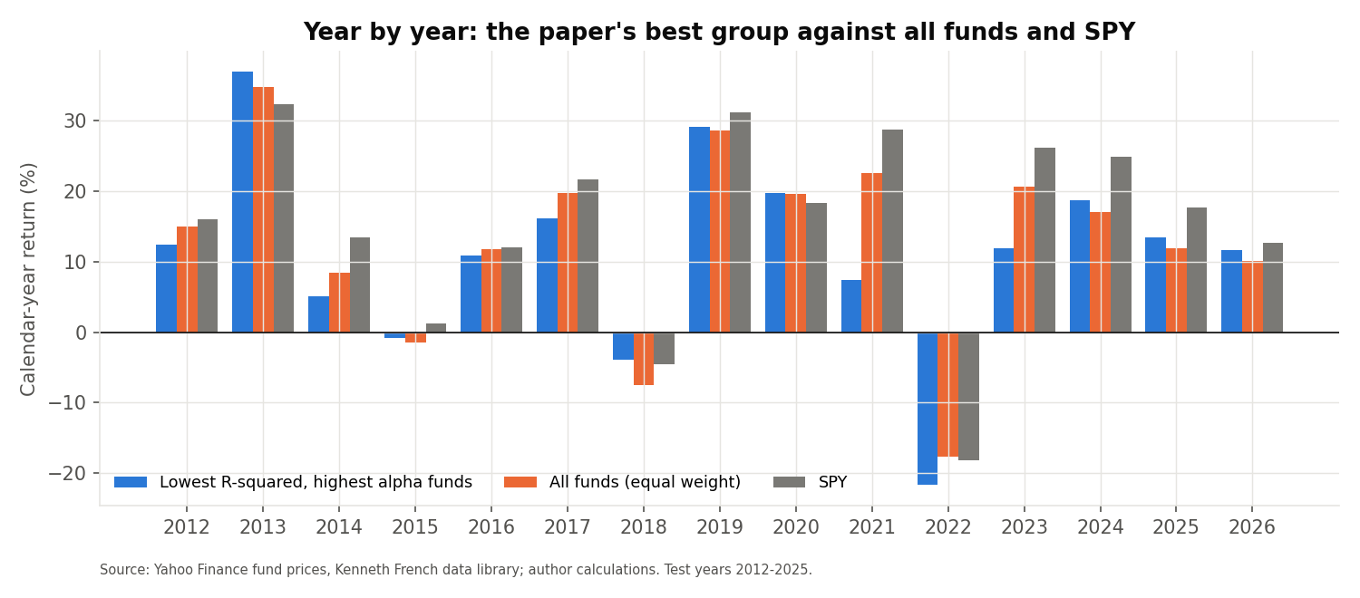
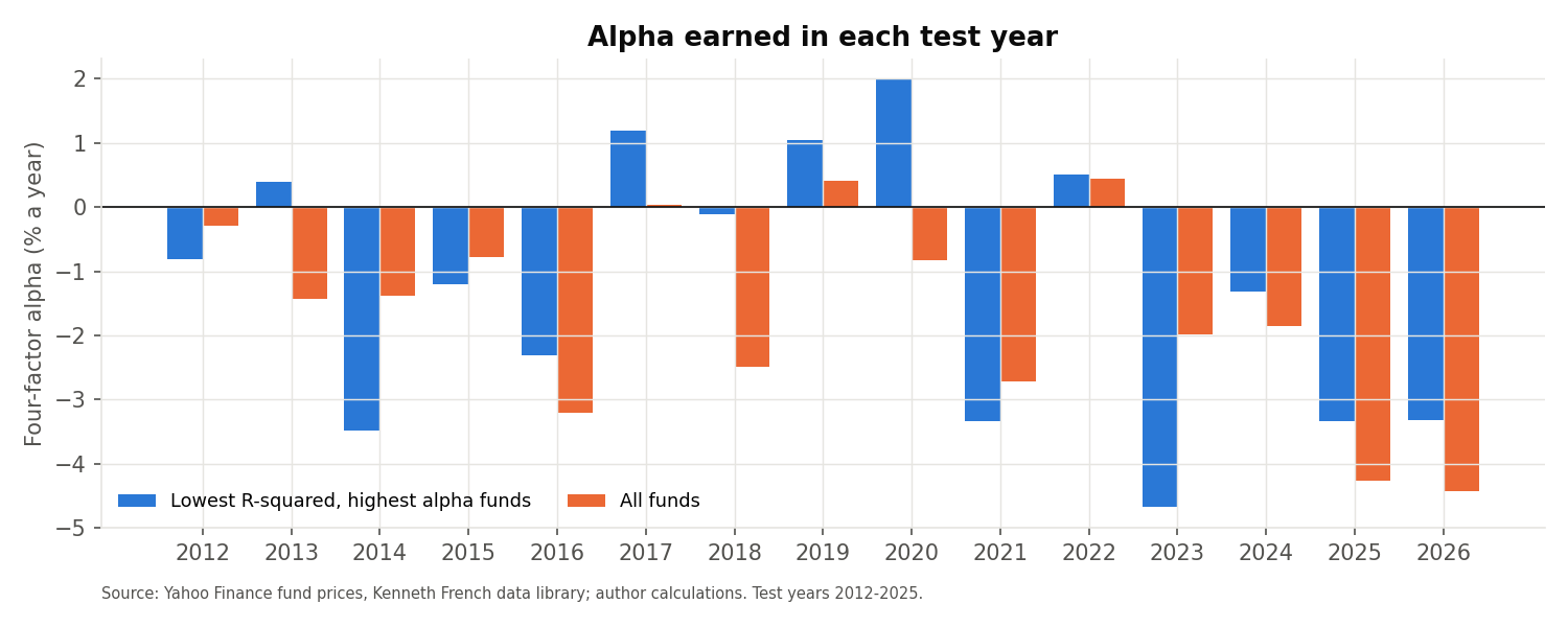
- The best group had a higher return than the average fund in 7 of 14 years and a higher alpha in 9. Its alpha was positive in only 5 years.
- Its average return was 2.0 percentage points a year below the average fund’s. The gap was widest in 2021, 2023, 2022; the group did better than the average fund in 2018, 2013, 2024.
- Fund returns are net of fund expenses, while SPY is a low-cost index fund, so SPY is a demanding comparison in a period when large US stocks led the market.
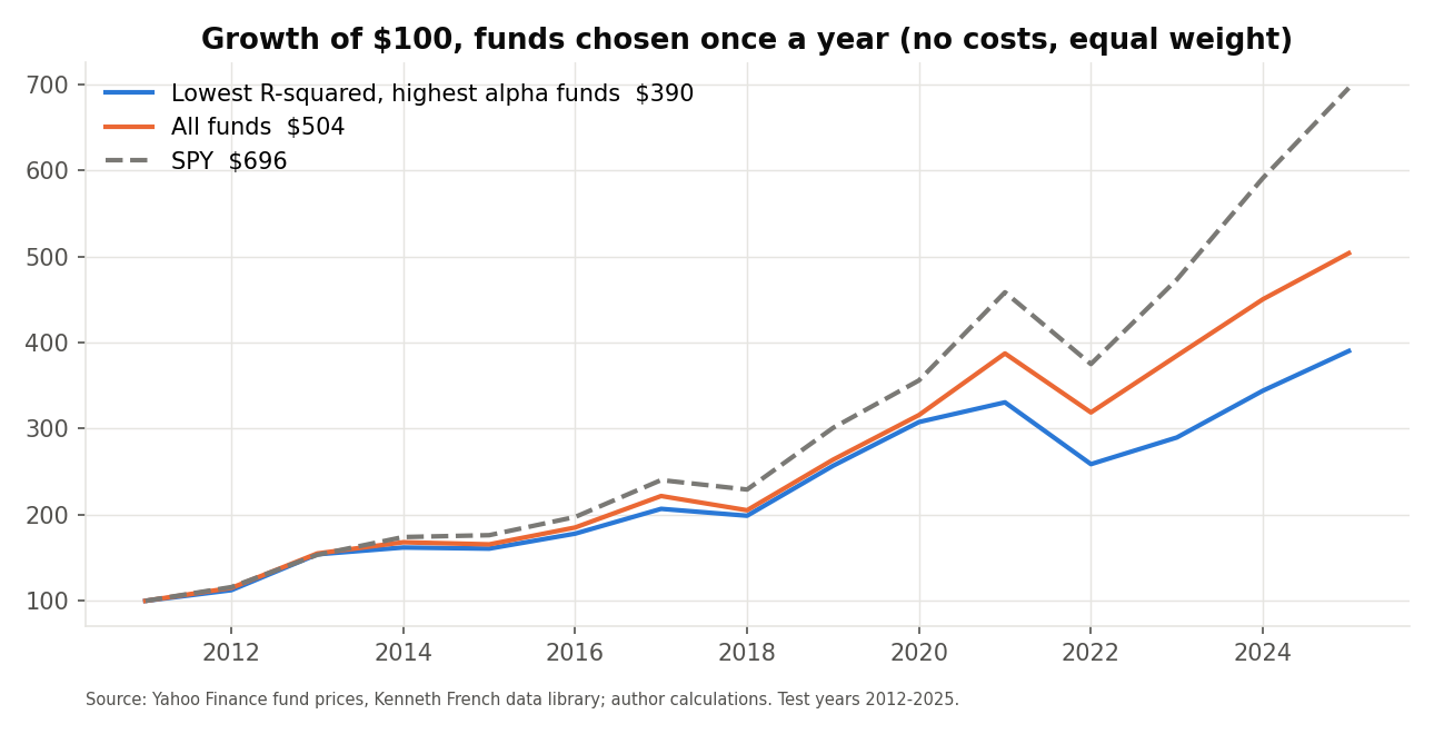
With funds chosen once a year, $100 became $390 in the best group, $504 across all funds and $696 in SPY, a compound rate of 10.21%, 12.24% and 14.86% a year over the 14.75 years.
2026 so far
The test year 2026 covers January to September only, so it is kept out of the tables above. Using the same rule on the 1,350 funds sorted with 2025 estimates, the lowest-R-squared, highest-alpha group (54 funds) had a four-factor alpha of −3.33% a year, against −4.43% for all funds. Over the nine months its average return was 11.68%, against 10.12% for all funds and 12.71% for SPY. These are partial-year figures and are not annualised for the returns.
Extension: a monthly long-short adaptation of the book’s rule
The book describes a monthly rotation of ETFs: buy the lowest-R-squared, highest-alpha group and sell the highest-R-squared, lowest-alpha group. The book applies the rule to ETFs and does not fix the rebalancing frequency; monthly is our choice. Open-end mutual funds generally cannot be sold short, so this is a simulation, not a tradeable strategy. Applied to the same funds (one regression a year of daily data, 252 days, estimated each month-end; equal weights; held one month; 10 bps cost on both legs on drift-adjusted turnover; no borrowing fee on the short leg) the result is below. Funds rebalance at the month-end close and earn the next month, from February 2012 to December 2025 (167 months), with 1,359 funds ranked each month and about 55 in each leg.
| CAGR | Volatility | Sharpe | Max drawdown | Monthly turnover | |
|---|---|---|---|---|---|
| R² × alpha long-short (the book’s rule) | −1.37% | 6.2% | −0.19 | −29.1% | 107% |
| Long leg only | 12.01% | 15.7% | 0.80 | −26.6% | 51% |
| Alpha-only long-short | −0.91% | 4.7% | −0.17 | −18.1% | 90% |
| R²-only long-short | −1.42% | 3.3% | −0.41 | −20.3% | 28% |
| All funds, equal weight | 11.75% | 14.9% | 0.82 | −24.5% | 2% |
| SPY | 14.58% | 13.9% | 1.05 | −23.9% | 0% |
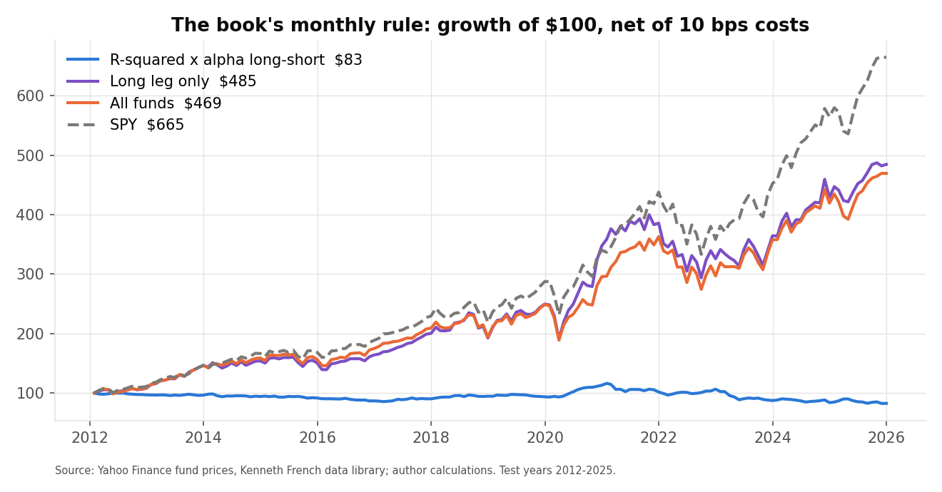
The long-short rule lost 1.37% a year after costs and 0.09% before costs. Its long leg matched the average fund and trailed SPY. Robustness checks, all on the same months:
- Estimation window of 126, 252 or 504 days: the long-short result ranged from −1.4% to −0.4% a year; no window was positive.
- Factor timing. The factor data are published with a delay. Lagging the estimation window by 0, 5 or 21 trading days, and executing at the next day’s close, gave −2.6% to −1.4% a year, benchmarks traded the same way.
- Costs and shorting. At 0, 10, 25 and 50 bps per unit traded the result was −0.1%, −1.4%, −3.2% and −6.3% a year; a short-borrowing fee of 1%, 2% or 5% a year would lower it to −2.4%, −3.3% and −6.2%.
- Is it alpha? Regressing the monthly long-short return on the same four factors gives an alpha of −2.11% a year (t-statistic −1.29), not distinguishable from zero. The long leg minus all funds has an alpha of 0.00% (t-statistic 0.00). The long leg alone, as a portfolio in excess of the risk-free rate, has a four-factor alpha of −1.76% a year (t-statistic −1.46), against −1.76% for all funds (t-statistic −3.57): the portfolio-level alpha, estimated from monthly portfolio returns.
- Subperiods. 2012-2019: long-short −0.8%, long leg 12.2%, all funds 12.2%, SPY 14.3% a year; 2020-2025: long-short −2.1%, long leg 11.7%, all funds 11.2%, SPY 15.0% a year.
Why might the effect have gone?
We did not test these; they are candidate explanations, in the order we find most plausible given the evidence above.
- A different period. The original sample ended in 2007; ours starts in 2012. In 2012 to 2025 the market itself (SPY) returned 14.86% a year, led by large US stocks, which is a demanding benchmark for funds of any kind.
- The signal may have been competed away. Once a pattern is published, funds and investors may adapt to it. The original study itself reports that the predictive power of R-squared was weaker in its early years and stronger later, so a change of regime is possible in either direction.
- Index-like funds. Even after removing funds named “index”, the typical fund here has an R-squared of 0.92. There is less cross-sectional spread to exploit.
Limitations of this replication
- Survivorship. Yahoo lists funds that exist today. Funds that closed or merged are missing.
- No point-in-time characteristics. No historical size, expense ratio, turnover, tenure or Active Share, and no size filter. Our proxy controls are current values.
- Sample construction. The fund list and the share-class merge use information through 2026, and every fund in the sample still has prices in September 2026, so the sample contains survivors only. We cannot say whether this raises or lowers the results.
- Versions of the original study. The design here follows the working paper. The published version reports its main portfolio tests on monthly returns with portfolio-level alphas; those are not replicated.
- 2026. The main tests stop at 2025. 2026 (January to September) is shown separately and has no independent R implementation.
- Share classes. One class per fund by return correlation, instead of an asset-weighted average of classes.
- Data quality. Yahoo prices contain errors. We removed funds with one-day moves above 30%; smaller errors may remain.
- Short test period. Fourteen test years. The year-level statistics rest on 14 observations.
- Inference. The original does not say how its t-statistics are computed. We use fund-year observations, which is generous because funds in the same year share market movements.
- Not replicated: the Active Share results, the alternative factor sets and the tests that need fund characteristics. The monthly extension has no independent R implementation.
Conclusion
Run on 1,362 Yahoo mutual funds from 2012 to 2025, the working-paper design of Amihud and Goyenko does not reproduce their main result in this sample. The funds with the lowest R-squared and highest past alpha did not earn a positive alpha (they earned −1.10% a year), R-squared showed no significant relationship with next-year alpha, and the book’s monthly long-short rule lost money after costs. R-squared still orders funds by information ratio in the direction they found, although with negative alphas that is partly a scaling effect. A different period, or a signal that has since been competed away, could explain the divergence, and we cannot say which.
Code
Each script reads the price panel and the Fama-French files, runs the regressions, the sorts and the regression tables, and writes CSV files. The shaded block is the code behind Eq. (365) to (368): the fund-year regression. The scripts, the fund list and the results files are in the GitHub repository.
"""Replication of the empirical design of Amihud and Goyenko (2013), "Mutual Fund's R2 as Predictor of Performance",
Review of Financial Studies 26(3), on Yahoo US equity mutual funds, 2012-2026 (their sample: CRSP, 1990-2007).
Design (from the paper's Sections 2-5): for each fund and calendar year, regress daily excess returns on RM-Rf, SMB,
HML, MOM and their one-day lags (Dimson 1979); alpha, R2, RMSE, InfRatio = alpha/RMSE. R2 and alpha of year y-1 predict
alpha and InfRatio of year y. Tables reproduced: II, III (without fund-characteristic controls Yahoo does not have),
V (Fama-MacBeth), VIII (dependent 5x5 sort) and IX (independent 5x5 sort). Writes data/results_ag_python.json and
data/ag_fund_years.csv. Everything the article quotes comes from them."""
import json
import os
import re
from pathlib import Path

import numpy as np
import pandas as pd
import yfinance as yf

ROOT = Path(__file__).resolve().parents[1]
os.environ.setdefault("QS_RAW_DIR", str(ROOT / "data" / "raw"))
import r_squared as R
from ag_replication_lib import cluster_ols, design

D = ROOT / "data/funds"
MIN_PRIOR, MIN_TEST = 125, 50                      # daily observations needed in year y-1 and in year y (paper, Section 3)
meta = pd.read_csv(D / "yahoo_us_equity_funds_deduped.csv").set_index("ticker")
is_index = meta["name"].str.contains(r"\bindex\b|\bind\b", case=False, regex=True)   # paper: names with "index" or "ind"
tick = meta.index[~is_index].tolist()
px = pd.read_parquet(D / "fund_prices.parquet").loc["2010-06-01":, tick]
spy = R.spy_prices("2010-06-01")
ff = R.download_factors()
last = min(px.index[-1], ff.index[-1])
px, ff, spy = px.loc[:last], ff.loc[:last], spy.loc[:last]
fac = ff[R.FACTORS]
Z = pd.concat([fac, fac.shift(1).add_suffix("_L")], axis=1)          # current and one-lag factors (Dimson)
ret = R.pct(px)
d = ret.join(Z, how="inner").join(ff["RF"]).dropna(subset=list(Z.columns) + ["RF"])
yrs = d.index.year


def year_fit(y):
    """Per fund: alpha (annualised %), R2, RMSE (daily), SDR (daily), InfRatio, n days for calendar year y."""
    m = yrs == y
    X = np.column_stack([np.ones(m.sum()), d.loc[m, list(Z.columns)].to_numpy()])
    rf = d.loc[m, "RF"].to_numpy()
    Y = d.loc[m, tick].to_numpy() - rf[:, None]
    out = {}
    for j, t in enumerate(tick):
        ok = np.isfinite(Y[:, j])
        n = int(ok.sum())
        if n < MIN_TEST:
            continue
        A, y_ = X[ok], Y[ok, j]
        b = np.linalg.lstsq(A, y_, rcond=None)[0]
        e = y_ - A @ b
        ssr, sst = float(e @ e), float(((y_ - y_.mean()) ** 2).sum())
        rmse = np.sqrt(ssr / (n - A.shape[1]))
        out[t] = (b[0] * 252 * 100, 1 - ssr / sst, rmse, y_.std(ddof=1), b[0] / rmse, n)
    return pd.DataFrame(out, index=["alpha", "r2", "rmse", "sdr", "ir", "n"]).T


fits = {y: year_fit(y) for y in range(2011, 2027)}
rows = []
for y in range(2012, 2027):
    a, b = fits[y - 1], fits[y]
    j = a[a.n >= MIN_PRIOR].join(b, lsuffix="_p", rsuffix="")
    j = j.dropna(subset=["alpha"])
    j["year"], j["fund"] = y, j.index
    rows.append(j)
fy = pd.concat(rows, ignore_index=True)
LAST = 2025                                                                       # main sample 2012-2025; 2026 (Jan-Sep) is reported separately
fy26 = fy[fy.year == 2026]
fy = fy[fy.year <= LAST]
n_before = len(fy)
lo, hi = fy["r2_p"].quantile(0.01), fy["r2_p"].quantile(0.99)                     # symmetric 1% trim of R2 (paper, Section 3), main sample
fy = fy[(fy.r2_p >= lo) & (fy.r2_p <= hi)].reset_index(drop=True)
fy26 = fy26[(fy26.r2_p >= lo) & (fy26.r2_p <= hi)].reset_index(drop=True)
for _d in (fy26,):
    _d["tr2"] = np.log(np.sqrt(_d.r2_p) / (1 - np.sqrt(_d.r2_p)))
fy["tr2"] = np.log(np.sqrt(fy.r2_p) / (1 - np.sqrt(fy.r2_p)))
fy["style"] = meta.loc[fy.fund, "yahoo_category"].to_numpy()
fy.to_csv(ROOT / "data/ag_fund_years.csv", index=False)


# ---------- helpers ----------
def panel(dep, cols, df):
    X = design(df, cols)
    b, se, r2 = cluster_ols(df[dep].to_numpy(float), X, df["fund"].to_numpy())
    return {"coef": {c: float(b[1 + i]) for i, c in enumerate(cols)}, "t": {c: float(b[1 + i] / se[1 + i]) for i, c in enumerate(cols)},
            "n_funds": int(df.fund.nunique()), "n_fund_years": int(len(df)), "r2": float(r2)}


def welch(a, b):
    return float((a.mean() - b.mean()) / np.sqrt(a.var(ddof=1) / len(a) + b.var(ddof=1) / len(b)))


def sort_tables(df, dep, lag, independent):
    """5x5 tables: rows = quintile of `lag` (alpha_p or ir_p), columns = quintile of R2_p. Cell = mean of year-y `dep`."""
    df = df.copy()
    df["qr"] = 0
    df["qa"] = 0
    for y, g in df.groupby("year"):
        rr = g["r2_p"].rank(method="first")
        qr = R.bin_of(rr, len(g))
        df.loc[g.index, "qr"] = qr
        if independent:
            df.loc[g.index, "qa"] = R.bin_of(g[lag].rank(method="first"), len(g))
        else:
            for q in range(1, 6):
                mem = g.index[qr == q]
                df.loc[mem, "qa"] = R.bin_of(df.loc[mem, lag].rank(method="first"), len(mem))
    cell = {}
    for a in range(1, 6):
        for q in range(1, 6):
            s = df.loc[(df.qa == a) & (df.qr == q), dep]
            cell[(a, q)] = (float(s.mean()), float(s.mean() / (s.std(ddof=1) / np.sqrt(len(s)))), int(len(s)))
    margin_a = {a: (float(df.loc[df.qa == a, dep].mean()), float(df.loc[df.qa == a, dep].mean() / (df.loc[df.qa == a, dep].std(ddof=1) / np.sqrt((df.qa == a).sum())))) for a in range(1, 6)}
    margin_r = {q: (float(df.loc[df.qr == q, dep].mean()), float(df.loc[df.qr == q, dep].mean() / (df.loc[df.qr == q, dep].std(ddof=1) / np.sqrt((df.qr == q).sum())))) for q in range(1, 6)}
    allm = float(df[dep].mean()), float(df[dep].mean() / (df[dep].std(ddof=1) / np.sqrt(len(df))))
    lowhigh = {a: (float(df.loc[(df.qa == a) & (df.qr == 1), dep].mean() - df.loc[(df.qa == a) & (df.qr == 5), dep].mean()),
                   welch(df.loc[(df.qa == a) & (df.qr == 1), dep], df.loc[(df.qa == a) & (df.qr == 5), dep])) for a in range(1, 6)}
    lowhigh["All"] = (float(df.loc[df.qr == 1, dep].mean() - df.loc[df.qr == 5, dep].mean()), welch(df.loc[df.qr == 1, dep], df.loc[df.qr == 5, dep]))
    highlow = {q: (float(df.loc[(df.qa == 5) & (df.qr == q), dep].mean() - df.loc[(df.qa == 1) & (df.qr == q), dep].mean()),
                   welch(df.loc[(df.qa == 5) & (df.qr == q), dep], df.loc[(df.qa == 1) & (df.qr == q), dep])) for q in range(1, 6)}
    highlow["All"] = (float(df.loc[df.qa == 5, dep].mean() - df.loc[df.qa == 1, dep].mean()), welch(df.loc[df.qa == 5, dep], df.loc[df.qa == 1, dep]))
    # stricter inference: mean of the 15 annual averages of the Low-R2 / High-alpha cell and its t over years
    yearly = df[(df.qa == 5) & (df.qr == 1)].groupby("year")[dep].mean()
    ts = {"mean": float(yearly.mean()), "t": float(yearly.mean() / (yearly.std(ddof=1) / np.sqrt(len(yearly)))), "years": int(len(yearly))}
    return {"cell": {f"{a}_{q}": v for (a, q), v in cell.items()}, "margin_alpha": margin_a, "margin_r2": margin_r, "all": allm,
            "low_minus_high_r2": lowhigh, "high_minus_low_alpha": highlow, "ts_lowR2_highAlpha": ts, "df": df}


out = {"params": {"first_test_year": 2012, "last_test_year": LAST, "last_price_date": str(px.index[-1].date()), "last_factor_date": str(ff.index[-1].date()),
                  "funds_after_index_filter": len(tick), "index_named_excluded": int(is_index.sum()),
                  "pairs_before_trim": int(n_before), "pairs_after_trim": int(len(fy)), "r2_trim_low": float(lo), "r2_trim_high": float(hi),
                  "min_days_prior": MIN_PRIOR, "min_days_test": MIN_TEST}}
out["table1"] = {c: {"mean": float(fy[c].mean()), "median": float(fy[c].median()), "sd": float(fy[c].std()), "min": float(fy[c].min()), "max": float(fy[c].max())}
                 for c in ("r2_p", "alpha_p", "rmse_p", "sdr_p", "alpha", "ir")}
out["table1"]["n_funds"], out["table1"]["n_fund_years"] = int(fy.fund.nunique()), int(len(fy))
fy["alpha_lag"], fy["ir_lag"] = fy["alpha_p"], fy["ir_p"]
for tname, dep, lagc in (("table2", "alpha", "alpha_lag"), ("table3", "ir", "ir_lag")):
    t = {}
    for per, (a, b) in {"full": (2012, LAST), "early": (2012, 2018), "late": (2019, LAST)}.items():
        sub = fy[(fy.year >= a) & (fy.year <= b)]
        t[per] = {"tr2": panel(dep, ["tr2"], sub), "tr2_lag": panel(dep, ["tr2", lagc], sub),
                  "comp": panel(dep, ["rmse_p", "sdr_p"], sub), "comp_lag": panel(dep, ["rmse_p", "sdr_p", lagc], sub)}
    out[tname] = t
fm = {}
for dep in ("alpha", "ir"):
    for name, cols in (("tr2", ["tr2"]), ("tr2_comp", ["tr2", "rmse_p", "sdr_p"])):
        cl = [("alpha_lag" if dep == "alpha" else "ir_lag")]
        coefs = []
        for y, g in fy.groupby("year"):
            X = np.column_stack([np.ones(len(g)), g[cols + cl].to_numpy(float)])
            coefs.append(np.linalg.lstsq(X, g[dep].to_numpy(float), rcond=None)[0])
        C = np.array(coefs)
        mean, se = C.mean(0), C.std(0, ddof=1) / np.sqrt(len(C))
        names = ["const"] + cols + cl
        fm[f"{dep}_{name}"] = {n: {"mean": float(mean[i]), "t": float(mean[i] / se[i]), "pos_share": float((C[:, i] > 0).mean())} for i, n in enumerate(names)}
out["table5"] = fm
res_dep = sort_tables(fy, "alpha", "alpha_p", False)
res_ir = sort_tables(fy, "ir", "ir_p", False)
ind_dep = sort_tables(fy, "alpha", "alpha_p", True)
ind_ir = sort_tables(fy, "ir", "ir_p", True)
for k, v in (("table8_alpha", res_dep), ("table8_ir", res_ir), ("table9_alpha", ind_dep), ("table9_ir", ind_ir)):
    out[k] = {kk: vv for kk, vv in v.items() if kk != "df"}

# ---------- year by year: the Low-R2 / High-alpha portfolio (dependent sort) ----------
dfq = res_dep["df"]
yp = px.copy()
yp["SPY"] = spy
ye = yp.groupby(yp.index.year).tail(1)
ye.index = ye.index.year
yret = (ye / ye.shift(1) - 1) * 100                                         # calendar-year total return by fund and SPY
rows = []
for y in range(2012, 2027):
    g = dfq[dfq.year == y] if y <= LAST else sort_tables(fy26, "alpha", "alpha_p", False)["df"]
    port = g[(g.qr == 1) & (g.qa == 5)]
    short = g[(g.qr == 5) & (g.qa == 1)]
    allr = yret.loc[y, g.fund].astype(float)
    pr = yret.loc[y, port.fund].astype(float)
    sr = yret.loc[y, short.fund].astype(float)
    rows.append({"year": y, "n_funds": int(len(g)), "n_portfolio": int(len(port)),
                 "alpha_portfolio": float(port.alpha.mean()), "alpha_all": float(g.alpha.mean()),
                 "ret_portfolio": float(pr.mean()), "ret_all_funds": float(allr.mean()), "ret_spy": float(yret.loc[y, "SPY"]),
                 "ret_hiR2_lowalpha": float(sr.mean()), "ret_long_short": float(pr.mean() - sr.mean()),
                 "partial_year": bool(y == 2026)})
yy_all = pd.DataFrame(rows)
yy_all.to_csv(ROOT / "data/ag_yearly.csv", index=False)
yy = yy_all[yy_all.year <= LAST].reset_index(drop=True)
out["yearly"] = rows[:-1]
out["update_2026"] = rows[-1]
cum = pd.DataFrame({"low_r2_high_alpha": ((1 + yy.ret_portfolio / 100).cumprod() * 100).to_numpy(), "all_funds": ((1 + yy.ret_all_funds / 100).cumprod() * 100).to_numpy(),
                    "spy": ((1 + yy.ret_spy / 100).cumprod() * 100).to_numpy()}, index=yy.year.to_numpy())
out["annual_summary"] = {k: {"cagr_pct": float(((cum[k].iloc[-1] / 100) ** (1 / len(cum)) - 1) * 100),
                             "years_beating_all_funds": int((yy.ret_portfolio > yy.ret_all_funds).sum()) if k == "low_r2_high_alpha" else None}
                         for k in cum.columns}
cum.to_csv(ROOT / "data/ag_cum_annual.csv")
json.dump(out, open(ROOT / "data/results_ag_python.json", "w"), indent=1, default=str)
c = out["table8_alpha"]["cell"]
print("pairs", n_before, "->", len(fy), " funds", fy.fund.nunique())
print("Table VIII panel A (mean alpha_y %, t):")
for a in range(5, 0, -1):
    print(a, " ".join(f"{c[f'{a}_{q}'][0]:7.2f}({c[f'{a}_{q}'][1]:5.1f})" for q in range(1, 6)), " All", f"{out['table8_alpha']['margin_alpha'][a][0]:.2f}")
print("Low-High R2 by alpha quintile:", {k: round(v[0], 2) for k, v in out["table8_alpha"]["low_minus_high_r2"].items()})
print("yearly:\n", yy[["year", "n_portfolio", "alpha_portfolio", "alpha_all", "ret_portfolio", "ret_all_funds", "ret_spy"]].round(2).to_string(index=False))
print("TR2 coef (alpha, full):", out["table2"]["full"]["tr2"]["coef"], out["table2"]["full"]["tr2"]["t"])
# Independent R implementation of the Amihud and Goyenko (2013) design on Yahoo US equity funds (see python/ag_replication.py).
# For every fund and calendar year: regress daily excess returns on MKT, SMB, HML, MOM and their one-day lags; keep alpha
# (annualised %), R2, RMSE, InfRatio. Year y-1 R2 and alpha predict year y alpha. Writes data/ag_r_*.csv for verify.py.
# Run from the r_squared folder with QS_RAW_DIR=data/raw. Inputs: data/funds/ag_prices.csv (adjusted closes of the active funds).
suppressPackageStartupMessages({ library(data.table); library(sandwich) })
D <- "data/funds"; MIN_PRIOR <- 125; MIN_TEST <- 50

french_daily <- function(zip_name, cols) {
  raw <- Sys.getenv("QS_RAW_DIR"); zf <- file.path(raw, zip_name)
  if (!file.exists(zf)) zf <- file.path(raw, sub("_CSV.zip", "_TXT.zip", zip_name))
  lines <- readLines(unz(zf, unzip(zf, list = TRUE)$Name[1]), warn = FALSE)
  body <- gsub(",", " ", lines[grepl("^[0-9]{8}[, ]", lines)])
  f <- read.table(text = body, header = FALSE, col.names = c("date", cols))
  data.frame(date = as.Date(as.character(f$date), "%Y%m%d"), f[, -1, drop = FALSE] / 100)
}
f3 <- french_daily("F-F_Research_Data_Factors_daily_CSV.zip", c("MKT", "SMB", "HML", "RF"))
fm <- french_daily("F-F_Momentum_Factor_daily_CSV.zip", "MOM")
ff <- merge(f3, fm, by = "date")                      # days both files cover
px <- fread(file.path(D, "ag_prices.csv")); dates <- as.Date(px$Date); P <- as.matrix(px[, -1]); tick <- colnames(P)
last <- min(tail(dates, 1), tail(ff$date, 1)); keep <- dates <= last; dates <- dates[keep]; P <- P[keep, ]; ff <- ff[ff$date <= last, ]
FAC <- c("MKT", "SMB", "HML", "MOM")
Fm <- as.matrix(ff[, FAC]); Z <- cbind(Fm, rbind(NA, Fm[-nrow(Fm), ])); colnames(Z) <- c(FAC, paste0(FAC, "_L"))
ok_z <- complete.cases(Z) & !is.na(ff$RF)
ret <- rbind(NA, P[-1, ] / P[-nrow(P), ] - 1)         # simple daily returns; NA across price gaps
common <- intersect(as.character(dates), as.character(ff$date[ok_z]))
ri <- match(common, as.character(dates)); fi <- match(common, as.character(ff$date))
RET <- ret[ri, ]; ZZ <- Z[fi, ]; RF <- ff$RF[fi]; yrs <- as.integer(format(as.Date(common), "%Y"))

year_fit <- function(y) {
  m <- which(yrs == y); X <- cbind(1, ZZ[m, ]); Y <- RET[m, ] - RF[m]
  res <- matrix(NA_real_, length(tick), 6, dimnames = list(tick, c("alpha", "r2", "rmse", "sdr", "ir", "n")))
  for (j in seq_along(tick)) {
    ok <- is.finite(Y[, j]); n <- sum(ok); if (n < MIN_TEST) next
    A <- X[ok, ]; yy <- Y[ok, j]; b <- qr.solve(A, yy); e <- yy - A %*% b
    ssr <- sum(e^2); sst <- sum((yy - mean(yy))^2); rmse <- sqrt(ssr / (n - ncol(A)))
    res[j, ] <- c(b[1] * 252 * 100, 1 - ssr / sst, rmse, sd(yy), b[1] / rmse, n)
  }
  res
}
fits <- setNames(lapply(2011:2025, year_fit), 2011:2025)
rows <- lapply(2012:2025, function(y) {
  a <- fits[[as.character(y - 1)]]; b <- fits[[as.character(y)]]
  keep <- !is.na(a[, "alpha"]) & a[, "n"] >= MIN_PRIOR & !is.na(b[, "alpha"])
  data.frame(year = y, fund = tick[keep], alpha_p = a[keep, "alpha"], r2_p = a[keep, "r2"], rmse_p = a[keep, "rmse"],
             sdr_p = a[keep, "sdr"], ir_p = a[keep, "ir"], alpha = b[keep, "alpha"], ir = b[keep, "ir"])
})
fy <- do.call(rbind, rows)
lo <- quantile(fy$r2_p, 0.01); hi <- quantile(fy$r2_p, 0.99)       # symmetric 1% trim (type-7 quantiles, as pandas)
fy <- fy[fy$r2_p >= lo & fy$r2_p <= hi, ]; rownames(fy) <- NULL
fy$tr2 <- log(sqrt(fy$r2_p) / (1 - sqrt(fy$r2_p)))
cat_map <- fread(file.path(D, "yahoo_us_equity_funds_deduped.csv"))
fy$style <- cat_map$yahoo_category[match(fy$fund, cat_map$ticker)]
fwrite(fy, "data/ag_r_fund_years.csv")

bin_of <- function(rank, n) ceiling(rank * 5 / n)
sorted <- function(df, dep, lag, independent) {
  df$qr <- 0L; df$qa <- 0L
  for (y in unique(df$year)) {
    i <- which(df$year == y); qr <- bin_of(rank(df$r2_p[i], ties.method = "first"), length(i)); df$qr[i] <- qr
    if (independent) df$qa[i] <- bin_of(rank(df[[lag]][i], ties.method = "first"), length(i)) else
      for (q in 1:5) { m <- i[qr == q]; df$qa[m] <- bin_of(rank(df[[lag]][m], ties.method = "first"), length(m)) }
  }
  out <- expand.grid(alpha_q = 1:5, r2_q = 1:5)
  s <- function(x) c(mean(x), mean(x) / (sd(x) / sqrt(length(x))), length(x))
  v <- t(mapply(function(a, q) s(df[[dep]][df$qa == a & df$qr == q]), out$alpha_q, out$r2_q))
  out$mean <- v[, 1]; out$t <- v[, 2]; out$n <- v[, 3]; out
}
for (nm in c("dep", "ind")) for (dv in c("alpha", "ir")) {
  lag <- if (dv == "alpha") "alpha_p" else "ir_p"
  fwrite(sorted(fy, dv, lag, nm == "ind"), sprintf("data/ag_r_table%s_%s.csv", if (nm == "dep") "8" else "9", dv))
}
# Table II/III style panel regressions: year and style dummies, standard errors clustered by fund
panel <- function(dep, cols, df) {
  f <- as.formula(paste(dep, "~", paste(c(cols, "factor(year)", "factor(style)"), collapse = " + ")))
  m <- lm(f, df); V <- vcovCL(m, cluster = df$fund, type = "HC1")     # CR1 small-sample factor, as in the Python code
  data.frame(var = cols, coef = coef(m)[cols], t = coef(m)[cols] / sqrt(diag(V))[cols], n = nrow(df))
}
tabs <- rbind(cbind(spec = "alpha_tr2", panel("alpha", "tr2", fy)), cbind(spec = "alpha_comp_lag", panel("alpha", c("rmse_p", "sdr_p", "alpha_p"), fy)),
              cbind(spec = "ir_tr2_lag", panel("ir", c("tr2", "ir_p"), fy)))
fwrite(tabs, "data/ag_r_regressions.csv"); print(tabs)
cat("fund-years", nrow(fy), "funds", length(unique(fy$fund)), "\n")
References
Kakushadze, Z. and Serur, J. A. (2018). 151 Trading Strategies. Available at SSRN: https://ssrn.com/abstract=3247865. Source paper
Implemented here: Chapter 4 (Exchange-traded funds), §4.3 “Strategy: R-squared”, Eq. (365) to (369) and footnotes 50, 77, 78 and 79, pp. 63–64.
Amihud, Y. and Goyenko, R. (2013). Mutual fund’s R² as predictor of performance. The Review of Financial Studies, 26(3), 667–694. doi:10.1093/rfs/hhs182 Cited in the book; replicated here
Carhart, M. M. (1997). On persistence in mutual fund performance. The Journal of Finance, 52(1), 57–82. doi:10.1111/j.1540-6261.1997.tb03808.x Cited in the book
Dimson, E. (1979). Risk measurement when shares are subject to infrequent trading. Journal of Financial Economics, 7(2), 197–226. doi:10.1016/0304-405X(79)90013-8 Cited in Amihud and Goyenko
Fama, E. F. and French, K. R. (1993). Common risk factors in the returns on stocks and bonds. Journal of Financial Economics, 33(1), 3–56. doi:10.1016/0304-405X(93)90023-5 Cited in the book
Data: French, K. R., Data Library, Fama/French 3 Factors (daily) and Momentum Factor (daily). mba.tuck.dartmouth.edu/pages/faculty/ken.french/data_library.html. Fund prices: Yahoo Finance.
Educational content, not investment advice. Backtested results are not a forecast of future returns.