Executive summary
Section 4.6 of 151 Trading Strategies builds a long-only trend-following portfolio from ETFs: keep the funds with a positive past return, then weight them by that return (Eq. 371), by return per unit of volatility (Eq. 372) or by return per unit of variance (Eq. 373). We test it on ten ETFs covering stocks, bonds, real estate, gold and commodities, 2007 to 31 October 2026:
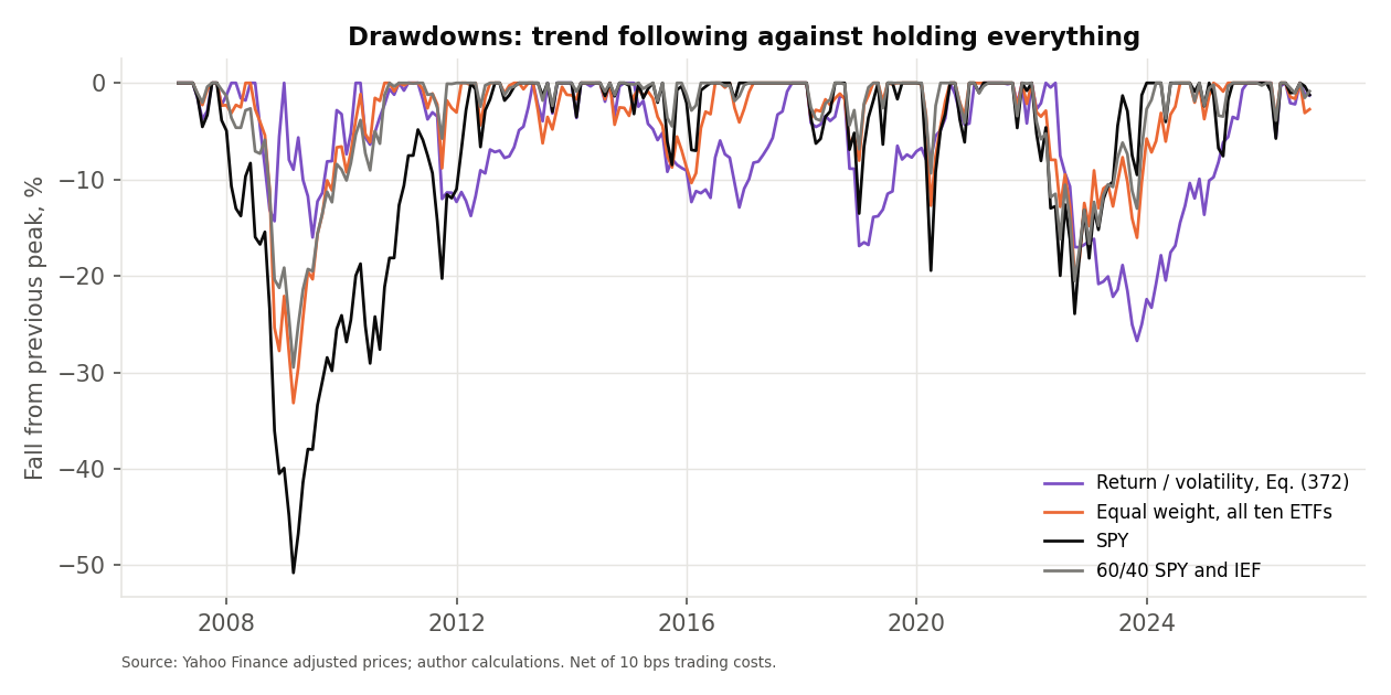
- Trend following cut the worst loss but not the return. The three weightings returned 5.01% to 6.70% a year net of costs, against 10.93% for the S&P 500 ETF and 6.27% for holding all ten equally. Their worst falls were −26.4% to −27.1%, against −50.8% for the S&P 500 ETF.
- The weighting changes the ranking only a little. Weighting by return earned the most and weighting by variance the least, with the Sharpe ratios close (0.57 to 0.62) and not clearly better than equal weighting (0.62).
- A cap on each weight helped most. Limiting any one fund to 35% (the book mentions bounds) raised the return of Eq. (371) to 7.7% and cut its worst fall to −17.3%, but it also holds more cash (8% of the portfolio on average against 3%), and we chose it after seeing the main results.
Introduction
An ETF gives exposure to a whole market, sector or asset class, so a handful of funds can diversify a portfolio. Trend following holds the ones that have been rising and avoids the ones that have not. The book (§4.6) sets out the rule and three ways to set the weights, but gives no data, no universe and no results, so everything below is our own implementation of the description.
Methodology
Data. Daily Yahoo Finance prices, adjusted for splits and distributions, for ten ETFs: SPY (US large companies), IWM (US small), EFA (developed markets outside the US), EEM (emerging markets), VNQ (US real estate), TLT (long Treasuries), IEF (medium Treasuries), LQD (corporate bonds), GLD (gold) and DBC (commodities). SHV (short Treasury bills) stands in for cash. The universe is our choice and the earliest common history starts in February 2007, so results begin in March 2007 and cover 236 months.
The rule. At each month-end, with T = 12 months, compute each fund’s cumulative return and keep only funds with a positive return and a price above their 200-day moving average. Weights are proportional to:
Ri is the return over the last T months and σi the volatility of daily returns over the previous 252 trading days. Each weighting is scaled so the weights sum to 1. If no fund qualifies, the portfolio holds the Treasury bill ETF. We trade at the month-end close, earn the following month, and charge 10 basis points on every dollar traded, including trades in the Treasury bill ETF and the trades needed to bring drifted weights back to target.
Differences from the book
| Element | Book, §4.6 | This article |
|---|---|---|
| Universe | Not specified | Ten ETFs of our choice (listed above) |
| Look-back | 6 to 12 months | 12 months in the main results; 6 and 9 tested |
| Moving average | Optional, 100 to 200 days | 200 days in the main results; also tested without |
| Volatility | “Historical volatility” | 252-day standard deviation of daily returns, annualised |
| Weight bounds | Mentioned, no value | 35% cap, a sensitivity run chosen after seeing the main results |
| Cash | Not specified | SHV when no fund qualifies; the weights otherwise sum to 1 |
| Costs and timing | Not specified | 10 bps on drift-adjusted turnover, counting the SHV leg; trade at the signal close (next-day execution also tested) |
Results and analysis
| Portfolio | Return, % a year | Volatility, % | Sharpe ratio (zero rate) | Sharpe ratio (over SHV) | Max drawdown, % | Monthly turnover, % |
|---|---|---|---|---|---|---|
| Weights by return, Eq. (371) | 6.7 | 11.6 | 0.62 | 0.48 | −26.4 | 45 |
| Return / volatility, Eq. (372) | 5.9 | 10.5 | 0.60 | 0.45 | −26.7 | 44 |
| Return / variance, Eq. (373) | 5.0 | 9.3 | 0.57 | 0.40 | −27.1 | 42 |
| Equal weight, all ten ETFs | 6.3 | 10.9 | 0.62 | 0.47 | −33.2 | |
| S&P 500 ETF (SPY) | 10.9 | 15.4 | 0.75 | 0.65 | −50.8 | |
| 60/40 SPY and IEF | 8.1 | 9.4 | 0.87 | 0.70 | −29.5 | |
| Treasury bill ETF (SHV) | 1.6 | 0.6 | 2.68 | −0.3 |
March 2007 to 31 October 2026, 236 months. Trend portfolios use a 12-month look-back and the 200-day filter, net of 10 bps costs. Equal weight holds all ten ETFs and rebalances monthly with the same costs; the 60/40 portfolio holds SPY and IEF. The first Sharpe column uses a zero risk-free rate; the second subtracts the monthly SHV return.
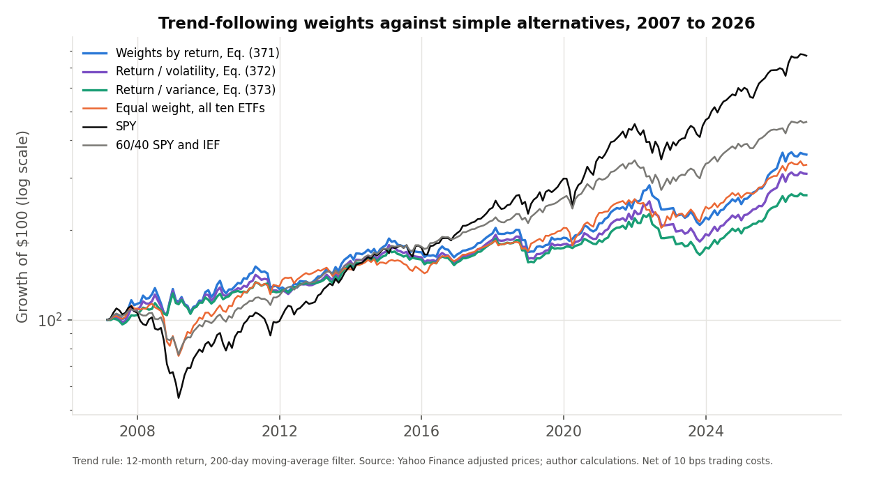
- Less risk, less return. Against the S&P 500 ETF, the trend portfolios gave up 4.2 to 5.9 points of annual return and roughly halved the worst fall: it was between −26.4% and −27.1%, against −50.8%. Over this period US stocks outperformed the diversified mixes, and trend following held a diversified mix.
- Little to separate the weightings. Weighting by return (Eq. 371) earned 6.70%, return per unit of volatility (Eq. 372) 5.90% and return per unit of variance (Eq. 373) 5.01%. Dividing by volatility or variance tilts the portfolio toward lower-volatility funds by construction, which lowers volatility (9.3% against 11.6%) and also the return. Sharpe ratios are within 0.05 of each other.
- Not clearly better than holding everything. Equal weighting of all ten earned 6.27% with a −33.2% worst fall. Only weighting by return (Eq. 371) beat it on return (0.4 points more); the other two earned less. A simple 60/40 portfolio of stocks and bonds had a higher Sharpe ratio (0.87, or 0.70 over SHV) than any of the three (0.62 at most, or 0.48 over SHV).
- Turnover is moderate: about 45% of the portfolio is traded each month, costing roughly 0.6 points a year; the portfolio held 5.7 funds on average and was fully in cash in 3% of months.
Is it robust?
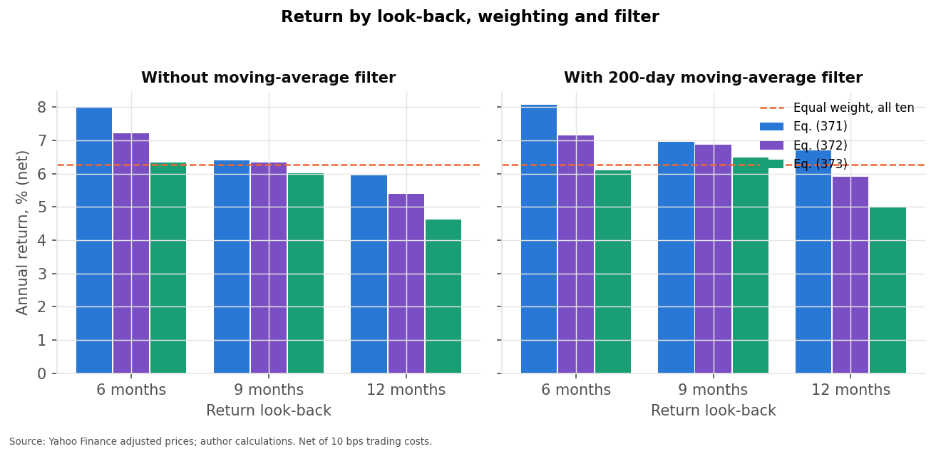
We re-ran 18 combinations of look-back (6, 9, 12 months), moving-average filter (on or off) and weighting. Net returns ranged from 4.6% to 8.1% a year, worst falls from −22.3% to −28.7%, and 12 of the 18 had a higher Sharpe ratio than equal weighting. The 12-month look-back, the one we report, did worse than the 6-month look-back in 6 of the 6 pairings of filter and weighting, so the main choice was not the best. Details are in the dropdown below; these are not 18 independent confirmations.
Capping weights. The book notes that bounds can limit overweighting. Capping each fund at 35% raised the return to 7.7% (Eq. 371), 7.0% (Eq. 372) and 6.4% (Eq. 373), with Sharpe ratios of 0.79 to 0.79 and worst falls of −17.3% to −13.8%. The cap also forces cash when fewer than three funds qualify: the portfolio held some SHV in 14% of months (against 3% uncapped) and 8% on average, so part of the lower drawdown comes from less market exposure, not better allocation among the funds. Because we added the cap after seeing the main results, and one run covers one period, we treat this as a hypothesis for further testing, not as a better strategy.
All 18 settings
| Setting | Return, % a year | Volatility, % | Sharpe ratio | Max drawdown, % | Turnover, % | Held | Cash, % of months |
|---|---|---|---|---|---|---|---|
| 6 months, no 200-day filter, Eq. (371) | 8.0 | 11.9 | 0.70 | −22.4 | 48 | 6.6 | 1 |
| 6 months, no 200-day filter, Eq. (372) | 7.2 | 10.8 | 0.70 | −22.4 | 48 | 6.6 | 1 |
| 6 months, no 200-day filter, Eq. (373) | 6.3 | 9.6 | 0.69 | −22.3 | 48 | 6.6 | 1 |
| 6 months, with 200-day filter, Eq. (371) | 8.1 | 12.0 | 0.71 | −24.5 | 50 | 6.1 | 1 |
| 6 months, with 200-day filter, Eq. (372) | 7.2 | 10.9 | 0.69 | −24.8 | 50 | 6.1 | 1 |
| 6 months, with 200-day filter, Eq. (373) | 6.1 | 9.8 | 0.66 | −25.1 | 50 | 6.1 | 1 |
| 9 months, no 200-day filter, Eq. (371) | 6.4 | 11.8 | 0.59 | −28.7 | 38 | 6.6 | 0 |
| 9 months, no 200-day filter, Eq. (372) | 6.3 | 10.4 | 0.64 | −23.4 | 38 | 6.6 | 0 |
| 9 months, no 200-day filter, Eq. (373) | 6.0 | 9.1 | 0.69 | −23.5 | 37 | 6.6 | 0 |
| 9 months, with 200-day filter, Eq. (371) | 7.0 | 11.4 | 0.65 | −25.1 | 44 | 5.9 | 2 |
| 9 months, with 200-day filter, Eq. (372) | 6.9 | 10.2 | 0.70 | −25.4 | 43 | 5.9 | 2 |
| 9 months, with 200-day filter, Eq. (373) | 6.5 | 9.1 | 0.74 | −25.8 | 42 | 5.9 | 2 |
| 12 months, no 200-day filter, Eq. (371) | 5.9 | 11.9 | 0.55 | −26.9 | 33 | 6.8 | 0 |
| 12 months, no 200-day filter, Eq. (372) | 5.4 | 10.6 | 0.55 | −23.5 | 31 | 6.8 | 0 |
| 12 months, no 200-day filter, Eq. (373) | 4.6 | 9.3 | 0.53 | −23.9 | 29 | 6.8 | 0 |
| 12 months, with 200-day filter, Eq. (371) | 6.7 | 11.6 | 0.62 | −26.4 | 45 | 5.7 | 3 |
| 12 months, with 200-day filter, Eq. (372) | 5.9 | 10.5 | 0.60 | −26.7 | 44 | 5.7 | 3 |
| 12 months, with 200-day filter, Eq. (373) | 5.0 | 9.3 | 0.57 | −27.1 | 42 | 5.7 | 3 |
Net of 10 bps, same 236 months. “Held” is the average number of funds held; “Cash” the share of months with no fund qualifying.
Next-day execution
The main results trade at the month-end close that produces the signal, a best case. Trading instead at the close of the next trading day earned 5.9% (Eq. 371), 5.1% (Eq. 372) and 4.2% (Eq. 373), up to 0.8 points a year below the main results, with Sharpe ratios of 0.49 to 0.55 (zero rate).
Trading costs
For Eq. (372) with the 12-month look-back and moving-average filter, the net return is 6.5% with no costs, 5.9% at 10 basis points, 5.1% at 25 and 3.7% at 50. Funds such as DBC and EEM trade with wider spreads than SPY, so 10 basis points may flatter the portfolio.
Limitations of this replication
- No original results. The book gives the rule but no data, universe or numbers, so this is one implementation of its description, not a reproduction of published returns.
- Short, single history. 236 months with one major crash (2008); the period favours US stocks. The universe is ours and the earliest data (DBC) limits the start to 2007.
- Survivors. All ten funds still trade; funds that closed are not included.
- Execution and costs. Trades at the month-end close, flat 10 bps, no taxes, no bid-ask spread differences, no market impact; cash is held in SHV, which earns its own return, pays the same 10 bps when traded and carries some interest-rate risk.
- Parameter choices. The main settings (12 months, 200 days, 252-day volatility) were chosen from the book’s ranges before running, but the sensitivity table shows other choices would have done better; the 35% cap was added after the results.
- Verification. The R code independently reproduces the monthly returns of all 18 settings; the cap, the next-day test, the cost scenarios, benchmarks and charts are Python only.
Conclusion
Under our implementation, long-only multi-asset trend following reduced the worst loss from −50.8% (the S&P 500 ETF) to between −26.4% and −27.1% but earned 4.2 to 5.9 points a year less, and it was not clearly better than simply holding all ten funds or a 60/40 mix. The three weighting schemes behaved similarly. A cap on single-fund weights looks worth testing on other universes and periods. This is one historical implementation of the book’s description, on a small, chosen universe, not a reproduction of published results.
Code
Each script reads the daily prices, builds the signals and weights and runs all 18 settings. The shaded block is the weight calculation and the monthly backtest. The scripts and results are in the GitHub repository.
"""4.6 Strategy: Multi-asset trend following -- implementation of Kakushadze & Serur (2018), "151 Trading Strategies", Section 4.6, Eq. (371)-(373).

Each month-end: R_i = P_i(t)/P_i(t-T) - 1 over T months; keep ETFs with R_i > 0 and (optionally) P_i > its 200-day moving average;
weights w_i = g1*R_i (371), g2*R_i/sigma_i (372) or g3*R_i/sigma_i^2 (373), normalised to sum to 1 over the kept ETFs.
sigma_i = annualised standard deviation of daily returns over the previous 252 trading days. If no ETF qualifies the portfolio holds the Treasury bill ETF (cash).
Trade at the month-end close, earn the next month, pay costs on drift-adjusted turnover (as in the 4.1 article).
Writes data/results_python.json and data/monthly_returns.csv.
"""
import json
from pathlib import Path

import numpy as np
import pandas as pd

ROOT = Path(__file__).resolve().parents[1]
UNIVERSE = ["SPY", "IWM", "EFA", "EEM", "VNQ", "TLT", "IEF", "LQD", "GLD", "DBC"]
CASH = "SHV"
COST_BPS = 10
MA_DAYS, VOL_DAYS = 200, 252
MAIN = dict(T=12, ma=True, wt="371", cap=None)


def load():
    px = pd.read_csv(ROOT / "data/prices.csv", index_col=0, parse_dates=True)
    daily = px[UNIVERSE + [CASH]]
    pm = daily.resample("ME").last()
    # inception months: a fund has no price before it exists; resample keeps NaN
    pm = pm.where(daily.resample("ME").count() > 0)
    ret_d = daily[UNIVERSE].pct_change(fill_method=None)
    sig = ret_d.rolling(VOL_DAYS, min_periods=VOL_DAYS).std().resample("ME").last() * np.sqrt(252)
    ma_ok = (daily[UNIVERSE] > daily[UNIVERSE].rolling(MA_DAYS, min_periods=MA_DAYS).mean()).where(
        daily[UNIVERSE].rolling(MA_DAYS, min_periods=MA_DAYS).mean().notna()).resample("ME").last()
    return pm, sig, ma_ok


def load_exec():
    """Close of the first trading day after each month-end (next-day execution test), indexed by the month-end it follows."""
    px = pd.read_csv(ROOT / "data/prices.csv", index_col=0, parse_dates=True)[UNIVERSE + [CASH]]
    fm = px.resample("MS").first()
    fm.index = fm.index - pd.Timedelta(days=1)
    return fm


def cap_weights(w, cap):
    """Iteratively cap each weight at `cap`; weight that cannot be placed under the cap goes to cash."""
    w = w.copy()
    for _ in range(20):
        over = w > cap + 1e-12
        if not over.any():
            break
        excess = (w[over] - cap).sum(); w[over] = cap
        free = (w < cap - 1e-12) & (w > 0)
        if free.sum() == 0 or w[free].sum() <= 0:
            break
        w[free] += excess * w[free] / w[free].sum()
    return w


def weights(pm, sig, ma_ok, T, ma, wt, cap):
    rcum = pm[UNIVERSE] / pm[UNIVERSE].shift(T) - 1
    ok = rcum > 0
    if ma:
        ok = ok & ma_ok.fillna(False).astype(bool)
    ok = ok & sig.notna() & rcum.notna()
    raw = {"371": rcum, "372": rcum / sig, "373": rcum / sig ** 2, "ew": rcum * 0 + 1}[wt]
    raw = raw.where(ok, 0.0).clip(lower=0)
    s = raw.sum(axis=1)
    w = raw.div(s.where(s > 0), axis=0).fillna(0.0)
    if cap is not None:
        w = w.apply(lambda r: cap_weights(r, cap), axis=1)
    return w, rcum


def start_month(pm, sig):
    rcum = pm[UNIVERSE] / pm[UNIVERSE].shift(12) - 1
    return rcum.dropna(how="any").index[0]


def run(pm, sig, ma_ok, T=12, ma=True, wt="371", cap=None, cost_bps=COST_BPS, start=None, pm_ex=None):
    w, rcum = weights(pm, sig, ma_ok, T, ma, wt, cap)
    px = pm if pm_ex is None else pm_ex
    r = px[UNIVERSE].pct_change(fill_method=None)
    rc = px[CASH].pct_change(fill_method=None)
    wl = w.shift(1)                                   # trade at month-end t, earn t+1
    cash_w = (1 - wl.sum(axis=1)).clip(lower=0)
    gross = (wl * r).sum(axis=1, min_count=1) + cash_w * rc
    drift = wl * (1 + r)
    tot = drift.sum(axis=1) + cash_w * (1 + rc)
    drift = drift.div(tot, axis=0)
    drift_cash = cash_w * (1 + rc) / tot
    turn = (wl - drift.shift(1)).abs().sum(axis=1) + (cash_w - drift_cash.shift(1)).abs()   # includes the SHV leg
    first = pm.index[pm.index > start][0]             # first month earned = month after the first signal
    turn.loc[first] = wl.loc[first].sum() + cash_w.loc[first]   # initial purchase of the whole portfolio
    net = gross - turn * cost_bps / 1e4
    held = (wl > 0).sum(axis=1)
    out = pd.DataFrame({"gross": gross, "rf": rc, "net": net, "turnover": turn, "cash": cash_w, "held": held}).loc[first:]
    return out.dropna(subset=["net"]), w


def stats(ret, rf=None):
    ret = ret.dropna(); yrs = len(ret) / 12
    eq = np.r_[1.0, (1 + ret).cumprod().to_numpy()]
    dd = eq / np.maximum.accumulate(eq) - 1
    return dict(cagr=(eq[-1] ** (1 / yrs) - 1) * 100, vol=ret.std(ddof=1) * np.sqrt(12) * 100,
                sharpe=ret.mean() / ret.std(ddof=1) * np.sqrt(12),
                sharpe_rf=(np.nan if rf is None else ((ret - rf.reindex(ret.index)).mean() / (ret - rf.reindex(ret.index)).std(ddof=1) * np.sqrt(12))), maxdd=dd.min() * 100, months=len(ret),
                start=str(ret.index[0].date()), end=str(ret.index[-1].date()))


def main():
    pm, sig, ma_ok = load()
    start = start_month(pm, sig)
    res = {"universe": UNIVERSE, "cash": CASH}
    # benchmarks, on the same months
    r = pm[UNIVERSE].pct_change(fill_method=None)
    # true equal-weight: hold all ten every month
    wl = pd.DataFrame(1 / len(UNIVERSE), index=pm.index, columns=UNIVERSE)
    def fixed(wdf, name):
        wl = wdf.shift(1); gross = (wl * r).sum(axis=1, min_count=1)
        drift = wl * (1 + r); drift = drift.div(drift.sum(axis=1), axis=0)
        turn = (wl - drift.shift(1)).abs().sum(axis=1)
        f = wl.dropna(how="all").index[0]; f = max(f, ret_first(wl, start)); turn.loc[f] = wl.loc[f].sum()
        return (gross - turn * COST_BPS / 1e4).loc[f:].dropna()
    def ret_first(wl, st):
        return wl.index[wl.index > st][0]
    first = pm.index[pm.index > start][0]
    bm = {}
    bm["Equal weight, all ten"] = fixed(wl, "ew")
    spy = r["SPY"].loc[first:]; bm["SPY buy and hold"] = spy
    w6040 = pd.DataFrame(0.0, index=pm.index, columns=UNIVERSE); w6040["SPY"] = 0.6; w6040["IEF"] = 0.4
    bm["60/40 SPY and IEF, monthly"] = fixed(w6040, "6040")
    cashr = pm[CASH].pct_change(fill_method=None).loc[first:]; bm["Treasury bill ETF"] = cashr
    res["benchmarks"] = {k: stats(v, cashr) for k, v in bm.items()}
    rets = {k: v for k, v in bm.items()}
    # main variants and the sensitivity grid
    grid = {}; gridret = {}
    for T in (6, 9, 12):
        for ma in (False, True):
            for wt in ("371", "372", "373"):
                o, _ = run(pm, sig, ma_ok, T=T, ma=ma, wt=wt, start=start)
                s = stats(o["net"], cashr); s["gross_cagr"] = stats(o["gross"])["cagr"]; s["turnover"] = o["turnover"].mean() * 100
                s["avg_held"] = o["held"].mean(); s["cash_months_pct"] = (o["cash"] > 0.999).mean() * 100
                grid[f"T{T}|ma{int(ma)}|{wt}"] = s; gridret[f"T{T}|ma{int(ma)}|{wt}"] = o["net"]
                if T == 12 and ma:
                    rets[f"Eq.({ {'371': 371, '372': 372, '373': 373}[wt] })"] = o["net"]
    res["grid"] = grid; pd.DataFrame(gridret).to_csv(ROOT / "data/grid_returns_python.csv")
    caps = {}
    for wt in ("371", "372", "373"):
        o, _ = run(pm, sig, ma_ok, T=12, ma=True, wt=wt, cap=0.35, start=start)
        s = stats(o["net"], cashr); s["turnover"] = o["turnover"].mean() * 100; s["cash_months_pct"] = (o["cash"] > 0.999).mean() * 100
        s["avg_cash_pct"] = o["cash"].mean() * 100; s["cash_any_pct"] = (o["cash"] > 0.001).mean() * 100
        u, _ = run(pm, sig, ma_ok, T=12, ma=True, wt=wt, start=start)
        s["uncapped_avg_cash_pct"] = u["cash"].mean() * 100; s["uncapped_cash_any_pct"] = (u["cash"] > 0.001).mean() * 100
        caps[wt] = s
    res["cap35"] = caps
    costs = {}
    for c in (0, 10, 25, 50):
        o, _ = run(pm, sig, ma_ok, T=12, ma=True, wt="372", cost_bps=c, start=start)
        costs[str(c)] = stats(o["net"])["cagr"]
    res["costs_372"] = costs
    pmx = load_exec().reindex(pm.index)
    nd = {}
    for wt in ("371", "372", "373"):
        o, _ = run(pm, sig, ma_ok, T=12, ma=True, wt=wt, start=start, pm_ex=pmx)
        nd[wt] = stats(o["net"], cashr)
    res["next_day"] = nd
    # yearly returns for the three main variants and benchmarks
    df = pd.DataFrame(rets)
    df.to_csv(ROOT / "data/monthly_returns.csv")
    yr = (1 + df).groupby(df.index.year).prod() - 1
    res["yearly"] = (yr * 100).round(2).to_dict(orient="index")
    res["start"] = str(first.date())
    json.dump(res, open(ROOT / "data/results_python.json", "w"), indent=1, default=float)
    print(json.dumps({k: res[k] for k in ("benchmarks",)}, indent=1)[:1500])
    for k, v in grid.items():
        print(k, round(v["cagr"], 2), round(v["sharpe"], 2), round(v["maxdd"], 1), round(v["turnover"]), round(v["avg_held"], 1), round(v["cash_months_pct"]))


if __name__ == "__main__":
    main()
# Independent R implementation of the 4.6 multi-asset trend-following study (see python/trend.py). Writes data/trend_r_returns.csv: net monthly returns of the 18 grid cells.
suppressPackageStartupMessages(library(data.table))
UNIVERSE <- c("SPY", "IWM", "EFA", "EEM", "VNQ", "TLT", "IEF", "LQD", "GLD", "DBC"); CASH <- "SHV"; COST <- 10
px <- fread("data/prices.csv"); setnames(px, 1, "Date"); px[, Date := as.Date(Date)]; setorder(px, Date)
mkey <- format(px$Date, "%Y-%m"); mlab <- unique(mkey)
lastvalid <- function(x) tapply(x, factor(mkey, levels = mlab), function(v) { v <- v[!is.na(v)]; if (length(v)) v[length(v)] else NA_real_ })
cols <- c(UNIVERSE, CASH)
pm <- sapply(cols, function(cc) as.numeric(lastvalid(px[[cc]]))); rownames(pm) <- mlab
n <- nrow(pm)
d <- sapply(UNIVERSE, function(cc) { x <- px[[cc]]; c(NA, x[-1] / x[-length(x)] - 1) })
fsd <- function(x, k) { m1 <- frollmean(x, k); m2 <- frollmean(x^2, k); sqrt((m2 - m1^2) * k / (k - 1)) }
sig <- sapply(UNIVERSE, function(cc) as.numeric(lastvalid(fsd(d[, cc], 252) * sqrt(252))))
ma_ok <- sapply(UNIVERSE, function(cc) { x <- px[[cc]]; m <- frollmean(x, 200); as.numeric(lastvalid(ifelse(is.na(m), NA, as.numeric(x > m)))) })
lag <- function(m, k) rbind(matrix(NA, k, ncol(m)), m[seq_len(nrow(m) - k), , drop = FALSE])
rcum_for <- function(T) pm[, UNIVERSE] / lag(pm[, UNIVERSE], T) - 1
start_i <- which(apply(rcum_for(12), 1, function(r) all(!is.na(r))))[1]
r <- pm[, UNIVERSE] / lag(pm[, UNIVERSE], 1) - 1; rc <- pm[, CASH] / c(NA, pm[-n, CASH]) - 1
run <- function(T, ma, wt) {
  rcum <- rcum_for(T); ok <- !is.na(rcum) & rcum > 0 & !is.na(sig)
  if (ma) ok <- ok & !is.na(ma_ok) & ma_ok == 1
  raw <- switch(wt, "371" = rcum, "372" = rcum / sig, "373" = rcum / sig^2)
  raw[!ok | is.na(raw)] <- 0; raw[raw < 0] <- 0
  s <- rowSums(raw); w <- raw / ifelse(s > 0, s, NA); w[is.na(w)] <- 0
  wl <- rbind(NA, w[-n, ]); cw <- pmax(1 - rowSums(wl), 0)
  gross <- rowSums(wl * r) + cw * rc
  drift <- wl * (1 + r); tot <- rowSums(drift) + cw * (1 + rc); drift <- drift / tot; dc <- cw * (1 + rc) / tot
  turn <- rowSums(abs(wl - rbind(NA, drift[-n, ]))) + abs(cw - c(NA, dc[-n]))   # includes the SHV leg
  f <- start_i + 1; turn[f] <- sum(wl[f, ]) + cw[f]
  (gross - turn * COST / 1e4)[f:n]
}
out <- list(); idx <- (start_i + 1):n
for (T in c(6, 9, 12)) for (ma in c(0, 1)) for (wt in c("371", "372", "373")) out[[sprintf("T%d|ma%d|%s", T, ma, wt)]] <- run(T, ma == 1, wt)
o <- as.data.table(out); o[, month := rownames(pm)[idx]]; fwrite(o, "data/trend_r_returns.csv"); cat("done", nrow(o), "months\n")
References
Kakushadze, Z. and Serur, J. A. (2018). 151 Trading Strategies. Available at SSRN: https://ssrn.com/abstract=3247865. Source paper
Implemented here: Chapter 4 (Exchange-traded funds), §4.6 “Strategy: Multi-asset trend following”, Eq. (371)–(373), p. 65 and footnote 83.
Data: Yahoo Finance daily prices for the ETFs listed in the repository.