Summary
This article implements Section 4.4 of Kakushadze & Serur (2018), 151 Trading Strategies. The section builds a mean-reversion strategy for ETFs from the Internal Bar Strength (IBS) of the previous day: where the close sits within the day’s range. An ETF that closed near its low is “cheap”, one that closed near its high is “rich”. The book’s source is Pagonidis (2014), The IBS Effect: Mean Reversion in Equity ETFs, which tested the idea on 33 ETFs up to 5 December 2013. We replicate that study on Yahoo Finance data for 31 of the same ETFs, first over the same window and then on the 13 years since.
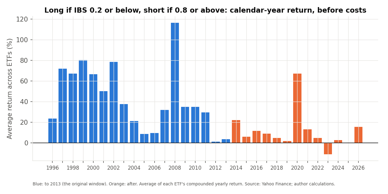
The original result replicates. To 5 December 2013, the average next-day return after an IBS in the lowest bucket (0 to 0.2) was 0.353%, and after the highest bucket (0.8 to 1) −0.134%; Pagonidis reports 0.350% and −0.126%. A rule that buys at an IBS of 0.2 or below and sells short at 0.8 or above earned 30.8% a year on average per ETF before costs, against “over 30%” in the original. The effect has weakened since: after 2013 the gap between the lowest and highest bucket is 0.19 percentage points a day, against 0.49 before, and the same rule earned 9.2% a year before costs. After costs of 5 basis points per trade it earned −0.1%.
The book’s own version, a daily dollar-neutral sort of ETFs by IBS into deciles, earned 38.6% a year before costs since 2013 but turns over its portfolio about 3.5 times a day, so the result depends almost entirely on the trading cost assumed: 16.4% at 2 basis points and −10.4% at 5. This is a backtest on free data; it is not a recommendation to trade.
The idea
Every trading day produces four prices: the open, the high, the low and the close. Internal Bar Strength asks where the close landed between the low and the high. If an ETF finished the day at its lowest price, its IBS is 0. At its highest price, 1. Pagonidis describes it as a one-period stochastic oscillator. The conjecture is that moves to the extremes of the day’s range are partly over-reactions to news or flows, and are partly reversed the next day.
Section 4.4 of the book describes the cross-sectional use: sort a universe of ETFs by IBS and, in a dollar-neutral portfolio, buy the bottom decile and sell the top decile, with equal weights or weights based on historical volatility. The book gives no data and no results, and cites Pagonidis (2014) for the evidence. We therefore replicate that study, and then test the book’s decile rule as an extension.
The research we replicate
Pagonidis uses daily open-high-low-close data for 33 ETFs, most of them iShares single-country funds (the list is in the repository), from each fund’s start to 5 December 2013. The analysis is:
- Five buckets. Each day is placed in one of five IBS buckets (0–0.2, 0.2–0.4, and so on), and the average close-to-close return of the next day is computed for each bucket and each ETF, with the probability that the next day is an up day.
- A simple strategy. Buy when the IBS is 0.2 or below, sell short when it is 0.8 or above, hold for one day, before costs.
- When it works. The effect is compared between high and low volatility days, high and low range days, bull and bear markets (positive or negative 200-day return), high and low volume days and days of the week, and the skewness of next-day returns is compared across buckets.
- As a filter. A long-only mean-reversion rule based on Cutler’s three-day RSI is compared with and without an IBS filter.
The headline findings are an average next-day return of 0.350% after the lowest bucket and −0.126% after the highest, an average strategy return above 30% a year before costs, and a stronger effect in volatile markets, in bear markets and on Mondays.
Data and methodology
We downloaded daily prices for the 33 ETFs from Yahoo Finance, adjusted for splits and dividends. IBS is a ratio inside one day, so the adjustment does not change it; close-to-close returns include dividends. Two of the 33 ETFs (GXG and RSX) have been delisted and Yahoo no longer provides their prices, which leaves 31. Daily bars where the high equals the low have no IBS and are skipped (3,754 bars in total, mostly early, thinly traded days), but they stay in the calendar so every return is a true one-day return. The data end on 17 November 2026.
Differences from the original sample
| Element | Original study | This article |
|---|---|---|
| Data source | CSI daily data | Yahoo Finance daily data, split- and dividend-adjusted |
| ETFs | 33 | 31 (GXG and RSX are no longer available) |
| Window | Each ETF’s start to 5 December 2013 | Same window, then 6 December 2013 to 17 November 2026 as a separate period |
| Volatility, volume and range splits | 20-day realised volatility split at the median; median over the sample, 500-day median for range | 20-day volatility split at the sample median; prior 500-day median for range and for volume (at least 250 days) |
| Strategy returns | Yearly returns by ETF, compounding not stated | Daily returns compounded within each year; the RSI rule is also shown as the arithmetic sum of daily returns, the original’s measure; no costs unless stated |
| RSI rule | Enter below 10, hold while RSI(3) is 40 or below; with the filter, enter or hold only if IBS is 0.5 or below | Same |
The first-listed date differs for some ETFs because Yahoo’s history begins at each fund’s launch. The original window contains about 3,373 trading days per ETF on average.
The maths
For an ETF with previous-day close PC, high PH and low PL (Eq. 370 of the book):
IBS is 0 when the close is the low of the day and 1 when it is the high. Footnote 81 of the book gives the symmetric version Y = IBS − 1/2, which runs from −1/2 to 1/2.
The bucket analysis conditions the next day’s return on which fifth of the 0 to 1 range today’s IBS falls in. With Pt the close on day t, the return after day t is:
The single-ETF strategy holds a position wt from the close of day t to the close of day t+1, with a cost c (in basis points) on each unit of change in the position:
wt = +1 if IBSt is 0.2 or below, −1 if it is 0.8 or above, and 0 otherwise.
The book’s version ranks N ETFs by IBS each day, buys the k = round(N/10) lowest and sells the k highest, with equal weights 1/k:
Each leg is $1, so gross exposure is $2. TOt is the sum of absolute changes in the weights between two days.
Results: the IBS effect replicates
Average close-to-close return on the day after each IBS bucket, as a percentage, averaged over the 31 ETFs:
| 1st (0–0.2) | 2nd | 3rd | 4th | 5th (0.8–1) | 1st − 5th | |
|---|---|---|---|---|---|---|
| Published average (to 5 Dec 2013) | 0.350 | 0.096 | 0.025 | −0.032 | −0.126 | 0.476 |
| Ours, to 5 Dec 2013 | 0.353 | 0.099 | 0.032 | −0.048 | −0.134 | 0.487 |
| Ours, after 5 Dec 2013 | 0.142 | 0.072 | 0.025 | −0.005 | −0.044 | 0.186 |
The published row is the average line of Pagonidis’s results. The window to 5 December 2013 reproduces it closely, including the asymmetry: the lowest bucket gains more than the highest bucket loses. In 29 of 31 ETFs the lowest bucket beat the highest in that window, and in 26 the difference is significant at the 1% level.
| 1st (0–0.2) | 2nd | 3rd | 4th | 5th (0.8–1) | 1st − 5th | |
|---|---|---|---|---|---|---|
| Published average | 56.8 | 52.7 | 51.3 | 49.9 | 46.2 | 10.5 |
| Ours, to 5 Dec 2013 | 57.2 | 53.1 | 51.7 | 49.7 | 46.4 | 10.8 |
| Ours, after 5 Dec 2013 | 54.4 | 52.8 | 50.9 | 51.1 | 50.3 | 4.1 |
Probability, in percent, that the next day is an up day. The published average gap between the lowest and highest bucket is 10.5 points.
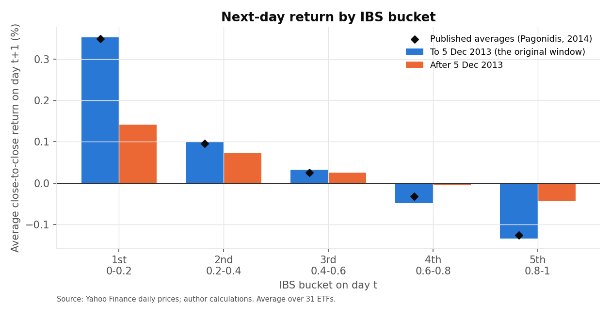
The effect is weaker since 2013. The lowest bucket still beats the highest in 29 of 31 ETFs, but the average gap has fallen from 0.49 to 0.19 percentage points, and the difference is significant at the 1% level in only 17 ETFs, against 26 before. The probability of an up day after the highest bucket is 50.3%, close to the unconditional probability, so the “sell” side has largely disappeared. The 1st to 5th gap in the probability of an up day is 4.1 points, against 10.8.
Results for each ETF
| ETF | Starts | To 2013: 1st | 5th | Rule %/yr | After: 1st | 5th | Rule %/yr |
|---|---|---|---|---|---|---|---|
| ECH | 2007 | 0.17 | 0.18 | −4.4 | −0.02 | 0.02 | −4.0 |
| EEM | 2003 | 0.43 | −0.01 | 23.3 | 0.16 | −0.06 | 12.3 |
| EFA | 2001 | 0.27 | −0.10 | 21.0 | 0.08 | −0.01 | 4.0 |
| EPHE | 2010 | 0.29 | −0.04 | 15.8 | 0.16 | −0.11 | 13.8 |
| EPI | 2008 | 0.40 | −0.32 | 43.9 | 0.22 | −0.11 | 19.0 |
| EPP | 2001 | 0.25 | −0.07 | 17.6 | 0.06 | −0.04 | 5.4 |
| EWA | 1996 | 0.51 | −0.29 | 65.1 | 0.07 | −0.06 | 6.5 |
| EWC | 1996 | 0.20 | −0.05 | 14.1 | 0.05 | 0.09 | −4.5 |
| EWD | 1996 | 0.38 | −0.17 | 37.0 | 0.06 | −0.03 | 3.9 |
| EWG | 1996 | 0.29 | −0.12 | 25.7 | 0.07 | −0.01 | 3.0 |
| EWH | 1996 | 0.54 | −0.35 | 57.8 | 0.18 | −0.09 | 14.4 |
| EWI | 1996 | 0.36 | −0.22 | 45.4 | 0.20 | −0.03 | 11.3 |
| EWJ | 1996 | 0.45 | −0.30 | 48.3 | 0.16 | −0.01 | 7.5 |
| EWL | 1996 | 0.49 | −0.26 | 60.2 | 0.07 | −0.02 | 4.9 |
| EWM | 1996 | 0.31 | −0.32 | 45.8 | 0.18 | −0.13 | 18.6 |
| EWO | 1996 | 0.33 | −0.17 | 32.7 | 0.16 | −0.03 | 9.4 |
| EWP | 1996 | 0.36 | −0.20 | 41.9 | 0.21 | −0.02 | 11.1 |
| EWQ | 1996 | 0.27 | −0.11 | 25.4 | 0.08 | −0.03 | 5.1 |
| EWS | 1996 | 0.54 | −0.38 | 63.7 | 0.11 | −0.02 | 6.2 |
| EWT | 2000 | 0.48 | −0.36 | 56.6 | 0.20 | 0.00 | 8.9 |
| EWU | 1996 | 0.35 | −0.20 | 35.4 | 0.05 | 0.00 | 1.7 |
| EWY | 2000 | 0.45 | −0.19 | 40.5 | 0.29 | −0.04 | 17.0 |
| EWZ | 2000 | 0.16 | 0.06 | 0.9 | 0.22 | −0.14 | 18.8 |
| EZA | 2003 | 0.49 | −0.09 | 33.2 | 0.21 | −0.11 | 16.5 |
| FXI | 2004 | 0.56 | −0.15 | 38.4 | 0.16 | −0.18 | 19.3 |
| IDX | 2009 | 0.28 | 0.13 | 2.2 | 0.14 | −0.15 | 18.2 |
| ILF | 2001 | 0.16 | 0.17 | −7.6 | 0.12 | −0.01 | 6.7 |
| IWM | 2000 | 0.25 | 0.00 | 13.1 | 0.12 | 0.00 | 4.7 |
| QQQ | 1999 | 0.25 | −0.07 | 17.6 | 0.25 | 0.04 | 7.1 |
| SPY | 1993 | 0.18 | −0.02 | 10.1 | 0.13 | 0.03 | 2.4 |
| THD | 2008 | 0.51 | −0.10 | 35.1 | 0.25 | −0.10 | 15.9 |
Average next-day return after the lowest and highest IBS bucket (%), and the average annual return of the long-short IBS rule before costs, by ETF, for the original window and after. “–” means fewer than 250 observations.
When does the effect work?
Pagonidis finds the effect is larger on high-volatility days, after high-range days, in bear markets, on high-volume days (for US ETFs) and on Mondays. The table shows the average gap in next-day return (lowest minus highest bucket, in percentage points) in each regime, for both periods.
| Regime on day t | To 5 Dec 2013 | After 5 Dec 2013 |
|---|---|---|
| High volatility | 0.70 | 0.25 |
| Low volatility | 0.25 | 0.11 |
| High range | 0.64 | 0.24 |
| Low range | 0.23 | 0.12 |
| Bear market (200-day return below 0) | 0.72 | 0.23 |
| Bull market | 0.35 | 0.18 |
| High volume | 0.50 | 0.23 |
| Low volume | 0.39 | 0.14 |
| After Monday | 0.77 | 0.33 |
| After Tuesday | 0.48 | 0.23 |
| After Wednesday | 0.38 | 0.21 |
| After Thursday | 0.49 | 0.04 |
| After Friday | 0.31 | 0.13 |
Average over ETFs with at least 20 observations in each of the two buckets. Volatility is the 20-day standard deviation of daily returns, split at each ETF’s median, range the day’s (high − low) / close against its prior 500-day median, trend the sign of the 200-day return.
- Volatility, range and trend. In the original window the gap is 0.70 points on high-volatility days against 0.25 on low-volatility days, and 0.72 in bear markets against 0.35 in bull markets, as the original reports. After 2013 the same ordering holds for volatility (0.25 against 0.11) and for the trend (0.23 against 0.18), at a smaller scale.
- Mondays. The gap is largest after Monday in both periods (0.77 and 0.33 points), and smallest after Friday in the original window (0.31); after 2013 Thursday is the weakest (0.04).
- Skewness. Next-day returns after the lowest bucket are positively skewed in the original window (0.66, against 0.65 reported) and negatively skewed after 2013 (−0.16).
The simple IBS strategy
Buy an ETF at the close when its IBS is 0.2 or below, sell it short when it is 0.8 or above, close the position the next day. Calendar-year returns, before costs, averaged over the ETFs:
| Average return per ETF, % a year | To 5 Dec 2013 | ETFs positive | After 5 Dec 2013 | ETFs positive |
|---|---|---|---|---|
| Before costs | 30.8 | 29 of 31 | 9.2 | 29 of 31 |
| 2 bps per unit traded | 26.1 | 27 of 31 | 5.4 | 26 of 31 |
| 5 bps per unit traded | 19.3 | 27 of 31 | −0.1 | 14 of 31 |
| 10 bps per unit traded | 8.7 | 21 of 31 | −8.6 | 1 of 31 |
Average over the 31 ETFs of each ETF’s compound annual return. Costs are charged per unit of position change, in basis points. The rule is in the market on 50% of days in the original window and 47% after.
The original window reproduces the “over 30% a year before costs” finding (30.8%), and the rule is profitable in 29 of 31 ETFs. After 2013 the average is 9.2% before costs and about zero at 5 basis points per unit traded. Pagonidis notes that trading costs make the rule on its own difficult to use, and that is the case here.
IBS as a filter for RSI
Pagonidis combines IBS with a longer-term rule: buy at the close when Cutler’s three-day RSI is below 10, hold while it is 40 or below, and, in the filtered version, hold only while IBS is 0.5 or below.
| Cutler’s RSI(3) rule | Sum of daily returns, % | Compounded, % | Days invested | Sum of daily returns, % | Compounded, % | Days invested |
|---|---|---|---|---|---|---|
| Without IBS filter | 121.9 | 266 | 750 | 20.3 | 20 | 735 |
| With IBS ≤ 0.5 filter | 119.4 | 263 | 378 | 30.4 | 36 | 368 |
The first three columns are to 5 December 2013, the last three after. Average over 31 ETFs, before costs. “Sum of daily returns” adds the returns of the days invested, the measure the original reports; “compounded” is the return of holding the strategy over the period. “Days invested” is the average number of trading days per ETF.
The filter halves the time invested in both periods (750 to 378 days per ETF to 5 December 2013; the original reports 725 to 412). Without the filter, the sum of daily returns is 121.9%, close to the 119.0% in the original. With the filter we get 119.4%, not the 128.6% reported: the filtered rule earned the same return in about half the days, but it did not add to it, and it was ahead in 13 of 31 ETFs. After 2013 the filter helps: 30.4% against 20.3% (compounded, 36% against 20%), ahead in 18 of 31 ETFs.
The book’s version: sorting ETFs by IBS into deciles
Every day, the 31 ETFs with a valid IBS (about 31 on average) are sorted by IBS; the bottom 3 are bought and the top 3 sold, with equal weights, $1 on each side, held for one day. Eligibility uses only information available at the close; if a selected ETF has no return the next day, its weight is spread over the other ETFs in that leg. Ties in IBS (a close exactly at the low or high is common) are broken by a ticker order that rotates every day, so that no ticker is favoured.
| Decile rule | CAGR % to 5 Dec 2013 | Sharpe | CAGR % after | Sharpe | Max drawdown % after |
|---|---|---|---|---|---|
| Before costs | 337.9 | 6.77 | 38.6 | 2.29 | −14.9 |
| 2 bps | 268.3 | 5.99 | 16.4 | 1.11 | −22.1 |
| 5 bps | 184.1 | 4.81 | −10.4 | −0.67 | −76.9 |
| 10 bps | 84.1 | 2.86 | −42.1 | −3.64 | −99.9 |
| Equal-weight all ETFs (reference) | 9.0 | 6.7 |
Long-short rule, daily, since the stated date. Costs are in basis points per unit of weight traded; the portfolio turns over about 3.5 units a day. Annual figures are compound annual growth rates.
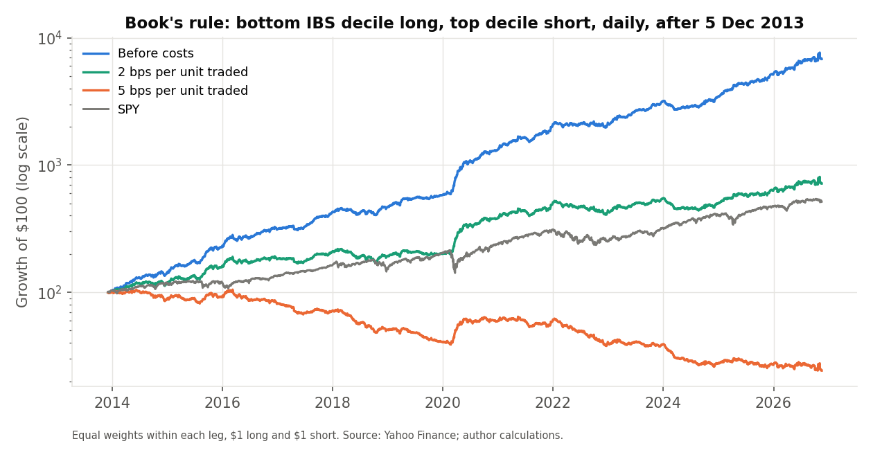
- Before costs the rule has a high Sharpe ratio (6.8 to 5 December 2013 and 2.3 after), because it holds the extremes of each day’s cross-section. The long leg earned 24.3% a year since 2013 and the short leg −11.2%.
- The cost assumption decides the result. At 2 basis points per unit traded the rule earned 16.4% a year since 2013, and at 5 basis points −10.4% with a maximum drawdown of −77%. The break-even cost is roughly 3.9 basis points. Fills at the close, which assume the final IBS can be traded on, and bid-ask spreads are outside this backtest. Costs here are on the trades needed to return to the target weights each day, allowing for the drift of holdings during the day; this changes the turnover by less than 0.1%, because the portfolio is almost entirely replaced each day. Adding a short-borrow fee of 1% a year lowers the result since 2013 by about 1.2 points a year (to 15.3% at 2 basis points).
- It is a high-turnover strategy on international ETFs. Many of the ETFs track foreign markets that are closed when the US close sets the IBS; Pagonidis suggests statistical arbitrageurs trading against these funds, which may be part of the effect. We have not tested this.
Why might the effect have weakened?
These are candidate explanations that we did not test.
- It has been published and traded. Pagonidis’s paper appeared in 2014, and short-term reversal strategies are widely known; the net edge on liquid ETFs may have been competed away.
- Different market structure. The spreads on liquid ETFs have narrowed and more trading takes place in the closing auction, which may reduce overreaction at the close.
- The sample. The post-2013 period has a long, strong bull market in US stocks; the original window includes 2000 to 2003 and 2008, years of high volatility, when the effect was strongest.
Limitations of this replication
- Different data vendor. Yahoo adjusted prices differ slightly from the data used in the original study, and the high and low of thinly traded early days may be unreliable.
- Survivors. Two of the original ETFs (GXG and RSX) are no longer available. The ETFs that remain are those that survived to today.
- Choices where the original is silent. Range and volume medians, compounding of yearly returns, the tie rule and the cost model are our choices, listed above.
- Annual returns. We report the average return per ETF a year (compounded within each year, 30.8% to 5 December 2013). The average of ETF-year returns in the original’s yearly table is about 29.4%, a related but different statistic, and we have not compared the two ETF by ETF and year.
- No costs in the replication tables. Costs appear only where stated, and no bid-ask spread, market impact or short-borrow cost is modelled.
- Cross-sectional dependence. The ETFs are correlated, so counting ETFs where an effect is significant overstates the number of independent tests.
- Verification. The R code independently reproduces the bucket tables, the probability of a positive day, the single-ETF rule and the decile rule; the regime splits, skewness and RSI rules are in Python only.
- Not replicated. The comparison of US and local ETFs, the developed and developing market split, the currency test and the figures for each bucket by ETF are in the original and not here.
Conclusion
The IBS effect in Pagonidis (2014) replicates: on 31 ETFs to 5 December 2013, next-day returns after low-IBS days were higher than after high-IBS days by 0.49 percentage points on average, and a simple long-short rule earned 30.8% a year before costs. Since then the gap has fallen to 0.19 points, the rule earned 9.2% before costs, and the book’s decile version earned 16.4% at 2 basis points and −10.4% at 5. Mean reversion at the daily frequency still shows up in the data; whether anything remains after trading costs depends on assumptions this backtest cannot settle.
Code
Each script reads the daily prices, computes IBS, the bucket tables and both strategies, and writes CSV files. The shaded block is the code behind the single-ETF strategy. The scripts and results files are in the GitHub repository.
"""4.4 Mean reversion: the IBS effect in equity ETFs. Replicates Pagonidis (2014), "The IBS Effect: Mean Reversion in Equity ETFs"
(NAAIM working paper) on Yahoo daily OHLC for the paper's ETFs, for the paper's own window (to 5 Dec 2013) and for the period after,
and adds the book's cross-sectional decile rule (Section 4.4, Eq. 370). Writes data/results_python.json and data/*.csv.
Definitions follow the paper; where it is silent the choice is noted in SPEC below and in the article."""
import json
from pathlib import Path

import numpy as np
import pandas as pd

ROOT = Path(__file__).resolve().parents[1]
CUT = pd.Timestamp("2013-12-05")            # last day of the paper's sample
SPEC = {"buckets": 5, "long_below": 0.2, "short_above": 0.8, "vol_window": 20, "range_window": 500, "range_min": 250, "bull_window": 200,
        "rsi_n": 3, "rsi_entry": 10, "rsi_hold": 40, "ibs_filter": 0.5, "decile_share": 0.1, "cost_bps": [0, 2, 5, 10]}

raw = pd.read_csv(ROOT / "data/ohlc_all.csv", parse_dates=["Date"], float_precision="round_trip")
# Days with High == Low (no range) or a close outside the range have no IBS; they stay in the calendar so returns are true one-day returns.
bad = raw[(raw.High <= raw.Low)]
raw = raw.copy()
raw["ibs"] = (raw.Close - raw.Low) / (raw.High - raw.Low).where(raw.High > raw.Low)
n_out = int(((raw.ibs < -1e-6) | (raw.ibs > 1 + 1e-6)).sum())
raw.loc[(raw.ibs < -1e-6) | (raw.ibs > 1 + 1e-6), "ibs"] = np.nan
raw["ibs"] = raw.ibs.clip(0, 1)
D = {}
for t, g in raw.groupby("ticker"):
    g = g.sort_values("Date").set_index("Date").copy()
    g["ret"] = g.Close.pct_change()
    g["nxt"] = g.ret.shift(-1)                                     # close-to-close return of the next trading day
    g["ndate"] = g.index.to_series().shift(-1)                      # date on which that return is earned
    g["vol10"] = g.ret.rolling(SPEC["vol_window"]).std()
    rng = (g.High - g.Low) / g.Close
    g["range_rel"] = rng / rng.rolling(SPEC["range_window"], min_periods=SPEC["range_min"]).median().shift(1)
    vm = g.Volume.rolling(SPEC["range_window"], min_periods=SPEC["range_min"]).median().shift(1)
    g["vol_rel"] = np.where(g.Volume > 0, g.Volume / vm, np.nan)
    g["trend"] = g.Close / g.Close.shift(SPEC["bull_window"]) - 1
    g["dow"] = g.index.dayofweek
    d = g.Close.diff()
    u, dn = d.clip(lower=0).rolling(SPEC["rsi_n"]).mean(), (-d.clip(upper=0)).rolling(SPEC["rsi_n"]).mean()
    g["rsi"] = np.where(dn == 0, 100.0, 100 - 100 / (1 + u / dn.replace(0, np.nan)))
    g.loc[u.isna() | dn.isna(), "rsi"] = np.nan
    D[t] = g
TICK = sorted(D)
PER = {"paper_window": lambda i: i <= CUT, "after": lambda i: i > CUT, "all": lambda i: i == i}
BUCKET = lambda x: np.minimum((x * SPEC["buckets"]).astype(int), SPEC["buckets"] - 1) + 1     # 1 = lowest IBS


def tt(x, mu=0.0):
    x = x.dropna()
    return float((x.mean() - mu) / (x.std(ddof=1) / np.sqrt(len(x)))) if len(x) > 2 and x.std(ddof=1) > 0 else np.nan


def welch(a, b):
    a, b = a.dropna(), b.dropna()
    return float((a.mean() - b.mean()) / np.sqrt(a.var(ddof=1) / len(a) + b.var(ddof=1) / len(b))) if len(a) > 2 and len(b) > 2 else np.nan


def valid(g, per):
    g = g[PER[per](g.index) & PER[per](pd.DatetimeIndex(g.ndate))]    # signal date AND the return date must both lie in the window
    return g[g.nxt.notna() & g.ibs.notna()]


out = {"params": {"spec": SPEC, "tickers": TICK, "n_tickers": len(TICK), "last_date": str(max(g.index.max() for g in D.values()).date()),
                  "rows_without_ibs_high_eq_low": int(len(bad)), "rows_ibs_outside_0_1_set_missing": n_out,
                  "first_dates": {t: str(D[t].index.min().date()) for t in TICK}}}

# ---------- Table 2: descriptive statistics ----------
t2 = {}
for per in PER:
    rows = {}
    for t in TICK:
        r = valid(D[t], per).nxt
        if len(r) > 30:
            rows[t] = {"n": int(len(r)), "mean": float(r.mean() * 100), "sd": float(r.std() * 100), "skew": float(r.skew()), "up": float((r > 0).mean() * 100)}
    t2[per] = rows
out["table2"] = t2

# ---------- Tables 3 and 4: next-day return and P(up) by IBS bucket ----------
t3, t4 = {}, {}
for per in PER:
    rows3, rows4 = {}, {}
    for t in TICK:
        g = valid(D[t], per)
        if len(g) < 250:
            continue
        b = BUCKET(g.ibs)
        mu = g.nxt.mean()
        r3 = {"n": [int((b == k).sum()) for k in range(1, 6)]}
        r3["mean"] = [float(g.nxt[b == k].mean() * 100) for k in range(1, 6)]
        r3["t_vs_avg"] = [tt(g.nxt[b == k], mu) for k in range(1, 6)]
        r3["diff_1_5"] = r3["mean"][0] - r3["mean"][4]
        r3["t_diff"] = welch(g.nxt[b == 1], g.nxt[b == 5])
        rows3[t] = r3
        up = (g.nxt > 0).astype(float)
        rows4[t] = {"up": [float(up[b == k].mean() * 100) for k in range(1, 6)]}
        rows4[t]["diff_1_5"] = rows4[t]["up"][0] - rows4[t]["up"][4]
    t3[per], t4[per] = rows3, rows4
out["table3"], out["table4"] = t3, t4


def avg_row(rows, key):
    return [float(np.mean([r[key][k] for r in rows.values()])) for k in range(5)]


out["table3_avg"] = {per: {"mean": avg_row(t3[per], "mean"), "diff_1_5": float(np.mean([r["diff_1_5"] for r in t3[per].values()])),
                           "n_etfs": len(t3[per]),
                           "n_sig_diff": int(sum(abs(r["t_diff"]) > 2.576 and r["diff_1_5"] > 0 for r in t3[per].values())),
                           "n_pos_diff": int(sum(r["diff_1_5"] > 0 for r in t3[per].values()))} for per in PER}
out["table4_avg"] = {per: {"up": avg_row(t4[per], "up"), "diff_1_5": float(np.mean([r["diff_1_5"] for r in t4[per].values()]))} for per in PER}

# ---------- conditional tables: volatility, range, trend, volume, weekday ----------
def cond_table(per, label, split):
    """Average over ETFs of the 1st and 5th bucket mean (raw and vol-adjusted) in each regime."""
    res = {}
    for reg in split["levels"]:
        a_raw, a_adj = [], []
        for t in TICK:
            g = valid(D[t], per)
            if len(g) < 500:
                continue
            m = split["fn"](g)
            if m is None:
                continue
            s = g[m == reg]
            b = BUCKET(s.ibs)
            adj = s.nxt / s.vol10
            if min((b == 1).sum(), (b == 5).sum()) < 20:
                continue
            a_raw.append((s.nxt[b == 1].mean() * 100, s.nxt[b == 5].mean() * 100))
            a_adj.append((adj[b == 1].mean(), adj[b == 5].mean()))
        if a_raw:
            r = np.array(a_raw)
            ad = np.array(a_adj)
            res[str(reg)] = {"n_etfs": len(a_raw), "b1": float(r[:, 0].mean()), "b5": float(r[:, 1].mean()), "diff": float((r[:, 0] - r[:, 1]).mean()),
                             "adj_b1": float(ad[:, 0].mean()), "adj_b5": float(ad[:, 1].mean()), "adj_diff": float((ad[:, 0] - ad[:, 1]).mean())}
    return res


def by_median(col):
    def fn(g):
        x = g[col]
        if x.notna().sum() < 500:
            return None
        return pd.Series(np.where(x.isna(), "na", np.where(x >= x.median() if col == "vol10" else x >= 1.0, "high", "low")), index=g.index)
    return fn


SPLITS = {"volatility": {"levels": ["high", "low"], "fn": by_median("vol10")},
          "range": {"levels": ["high", "low"], "fn": by_median("range_rel")},
          "trend": {"levels": ["bull", "bear"], "fn": lambda g: pd.Series(np.where(g.trend.isna(), "na", np.where(g.trend > 0, "bull", "bear")), index=g.index)},
          "volume": {"levels": ["high", "low"], "fn": by_median("vol_rel")},
          "weekday": {"levels": ["Mon", "Tue", "Wed", "Thu", "Fri"], "fn": lambda g: pd.Series(g.dow.map({0: "Mon", 1: "Tue", 2: "Wed", 3: "Thu", 4: "Fri"}).to_numpy(), index=g.index)}}
out["conditional"] = {per: {k: cond_table(per, k, v) for k, v in SPLITS.items()} for per in PER}

# ---------- skewness by bucket ----------
sk = {}
for per in PER:
    rows = []
    for t in TICK:
        g = valid(D[t], per)
        if len(g) < 500:
            continue
        b = BUCKET(g.ibs)
        rows.append([float(g.nxt[b == k].skew()) for k in range(1, 6)])
    sk[per] = [float(x) for x in np.nanmean(np.array(rows), axis=0)]
out["skew_by_bucket"] = sk

# ---------- Table 5: IBS long/short per ETF (long if IBS <= 0.2, short if >= 0.8), yearly compounded returns ----------
def pos_ibs(g):
    return pd.Series(np.where(g.ibs <= SPEC["long_below"], 1.0, np.where(g.ibs >= SPEC["short_above"], -1.0, 0.0)), index=g.index)


def strat_returns(g, pos, cost_bps=0.0):
    """Position set at the close of day t earns day t+1's close-to-close return; cost on the change of position."""
    p = pos.shift(1).fillna(0.0)                                  # position held during day t (decided at close t-1)
    gross = (p * g.ret).where(g.ret.notna(), 0.0)
    turn = (pos.shift(1).fillna(0) - pos.shift(2).fillna(0)).abs()
    return gross - turn * cost_bps / 1e4


yearly, summary = {}, {}
for t in TICK:
    g = D[t]
    r = strat_returns(g, pos_ibs(g))
    yearly[t] = {str(y): float(((1 + x).prod() - 1) * 100) for y, x in r.groupby(r.index.year)}
out["table5_yearly"] = yearly
_py = [v for t in TICK for y, v in yearly[t].items() if int(y) <= CUT.year and D[t].index[D[t].index.year == int(y)].size > 100]
out["table5_avg_etf_year_to_2013"] = float(np.mean(_py))
out["table5_avg_etf_year_to_2013_n"] = len(_py)
for per in PER:
    tot = []
    for t in TICK:
        g = D[t]
        m = PER[per](g.index)
        r = strat_returns(g, pos_ibs(g))[m]
        if len(r) < 250:
            continue
        yrs = len(r) / 252
        tot.append({"t": t, "cagr": float(((1 + r).prod() ** (1 / yrs) - 1) * 100), "in_mkt": float((pos_ibs(g)[m] != 0).mean() * 100)})
    summary[per] = {"avg_cagr": float(np.mean([x["cagr"] for x in tot])), "median_cagr": float(np.median([x["cagr"] for x in tot])),
                    "n_pos": int(sum(x["cagr"] > 0 for x in tot)), "n": len(tot), "avg_in_market_pct": float(np.mean([x["in_mkt"] for x in tot])),
                    "by_etf": {x["t"]: x["cagr"] for x in tot}}
out["ibs_strategy_gross"] = summary
costs = {}
for per in PER:
    costs[per] = {}
    for c in SPEC["cost_bps"]:
        v = []
        for t in TICK:
            g = D[t]
            m = PER[per](g.index)
            r = strat_returns(g, pos_ibs(g), c)[m]
            if len(r) >= 250:
                v.append(((1 + r).prod() ** (252 / len(r)) - 1) * 100)
        costs[per][str(c)] = {"avg_cagr": float(np.mean(v)), "n_pos": int(sum(x > 0 for x in v)), "n": len(v)}
out["ibs_strategy_costs"] = costs

# ---------- RSI(3) with and without the IBS filter ----------
def rsi_pos(g, filt):
    pos, prev = np.zeros(len(g)), 0.0
    for i, (rs, ib) in enumerate(zip(g.rsi.to_numpy(), g.ibs.to_numpy())):
        if np.isnan(rs):
            prev = 0.0
            continue
        ok = (not filt) or ib <= SPEC["ibs_filter"]
        prev = 1.0 if ok and (rs < SPEC["rsi_entry"] or (prev == 1.0 and rs <= SPEC["rsi_hold"])) else 0.0
        pos[i] = prev
    return pd.Series(pos, index=g.index)


rsi = {}
for per in PER:
    rows = []
    for t in TICK:
        g = D[t]
        m = PER[per](g.index)
        if m.sum() < 750:
            continue
        rr = {}
        for name, f in (("rsi", False), ("rsi_ibs", True)):
            p = rsi_pos(g, f)
            r = strat_returns(g, p)[m]
            rr[name] = {"total": float(((1 + r).prod() - 1) * 100), "sum": float(r.sum() * 100), "days": int((p[m] != 0).sum()), "in_mkt": float((p[m] != 0).mean() * 100), "trades": int(((p[m] == 1) & (p[m].shift(1).fillna(0) == 0)).sum())}
        rows.append({"t": t, **rr})
    rsi[per] = {"n": len(rows), "avg_sum_rsi": float(np.mean([x["rsi"]["sum"] for x in rows])), "avg_sum_filtered": float(np.mean([x["rsi_ibs"]["sum"] for x in rows])),
                "avg_days_rsi": float(np.mean([x["rsi"]["days"] for x in rows])), "avg_days_filtered": float(np.mean([x["rsi_ibs"]["days"] for x in rows])),
                "n_better_sum": int(sum(x["rsi_ibs"]["sum"] > x["rsi"]["sum"] for x in rows)),
                "avg_total_rsi": float(np.mean([x["rsi"]["total"] for x in rows])), "avg_total_filtered": float(np.mean([x["rsi_ibs"]["total"] for x in rows])),
                "avg_in_mkt_rsi": float(np.mean([x["rsi"]["in_mkt"] for x in rows])), "avg_in_mkt_filtered": float(np.mean([x["rsi_ibs"]["in_mkt"] for x in rows])),
                "avg_trades_rsi": float(np.mean([x["rsi"]["trades"] for x in rows])), "avg_trades_filtered": float(np.mean([x["rsi_ibs"]["trades"] for x in rows])),
                "n_better": int(sum(x["rsi_ibs"]["total"] > x["rsi"]["total"] for x in rows))}
out["rsi_filter"] = rsi

# ---------- the book's rule: cross-sectional decile sort on IBS, long bottom decile / short top decile ----------
ibs_w = pd.DataFrame({t: D[t].ibs for t in TICK})
ret_w = pd.DataFrame({t: D[t].ret for t in TICK})
nxt_w = ret_w.shift(-1)
# Eligibility uses only what is known at the close of the signal day (a valid IBS). A selected ETF with no next-day return
# (missing data, delisting) is counted below and its weight is spread over the other selected ETFs of the same leg.
cnt = ibs_w.notna().sum(axis=1)
k = np.maximum((cnt * SPEC["decile_share"]).round().astype(int), 1)
# ties (IBS of exactly 0 or 1 is common) are broken by a ticker order that rotates every day, so no ticker is systematically favoured
nT = len(TICK)
rot = (np.arange(nT)[None, :] + np.arange(len(ibs_w))[:, None]) % nT
ibs_t = ibs_w + pd.DataFrame(rot / nT * 1e-9, index=ibs_w.index, columns=ibs_w.columns)
rk = ibs_t.where(ibs_w.notna()).rank(axis=1, method="first")
long_m = rk.le(k, axis=0) & ibs_w.notna()
short_m = rk.gt(cnt - k, axis=0) & ibs_w.notna()
lw = long_m.div(long_m.sum(axis=1).replace(0, np.nan), axis=0)
sw = short_m.div(short_m.sum(axis=1).replace(0, np.nan), axis=0)
have = nxt_w.notna()


def leg_return(w):
    wa = w.where(have)
    return (wa * nxt_w).sum(axis=1, min_count=1) / wa.sum(axis=1).replace(0, np.nan)


rl, rs_ = leg_return(lw), leg_return(sw)
n_missing = int(((long_m | short_m) & ~have & nxt_w.index.to_series().lt(ret_w.index[-1]).to_numpy()[:, None]).sum().sum())
ew = nxt_w.where(ibs_w.notna()).mean(axis=1)
ok = cnt >= 10
dec = {}


def drift_turnover(w, r_leg):
    """Trades needed each day to go from yesterday's drifted holdings to today's target weights (one leg, weights sum to 1)."""
    prev_t = w.shift(1).fillna(0)
    drifted = prev_t.mul(1 + nxt_w.shift(1).fillna(0)).div((1 + r_leg.shift(1)).fillna(1), axis=0)
    return (w.fillna(0) - drifted).abs().sum(axis=1)


turn = ((lw.fillna(0) - lw.shift(1).fillna(0)).abs().sum(axis=1) + (sw.fillna(0) - sw.shift(1).fillna(0)).abs().sum(axis=1))
turn_d = drift_turnover(lw, rl) + drift_turnover(sw, rs_)
BORROW = 0.01                                                    # 1% a year on the short leg, charged daily, for the robustness scenario
for per in PER:
    m = pd.Series(PER[per](ibs_w.index), index=ibs_w.index) & ok & rl.notna() & rs_.notna()
    res = {}
    for c in SPEC["cost_bps"]:
        ls = (rl - rs_)[m] - turn.shift(0)[m] * c / 1e4
        yrs = m.sum() / 252
        res[str(c)] = {"cagr": float(((1 + ls).prod() ** (1 / yrs) - 1) * 100), "vol": float(ls.std() * np.sqrt(252) * 100), "sharpe": float(ls.mean() / ls.std() * np.sqrt(252)),
                       "mean_bp_day": float(ls.mean() * 1e4), "t": tt(ls), "max_dd": float(((1 + ls).cumprod() / (1 + ls).cumprod().cummax() - 1).min() * 100)}
        lsd = (rl - rs_)[m] - turn_d[m] * c / 1e4
        res[str(c) + "_drift"] = {"cagr": float(((1 + lsd).prod() ** (1 / yrs) - 1) * 100)}
        lsb = lsd - BORROW / 252
        res[str(c) + "_drift_borrow"] = {"cagr": float(((1 + lsb).prod() ** (1 / yrs) - 1) * 100)}
    res["long_leg_cagr"] = float(((1 + rl[m]).prod() ** (1 / (m.sum() / 252)) - 1) * 100)
    res["short_leg_cagr"] = float(((1 + rs_[m]).prod() ** (1 / (m.sum() / 252)) - 1) * 100)
    res["equal_weight_cagr"] = float(((1 + ew[m]).prod() ** (1 / (m.sum() / 252)) - 1) * 100)
    res["days"] = int(m.sum())
    res["avg_etfs"] = float(cnt[m].mean())
    res["avg_per_leg"] = float(k[m].mean())
    res["avg_daily_turnover"] = float(turn[m].mean())
    res["avg_daily_turnover_drift"] = float(turn_d[m].mean())
    res["selected_missing_next_return"] = n_missing if per == "all" else None
    dec[per] = res
out["decile_rule"] = dec
spy = D["SPY"].ret
okk = ok & rl.notna() & rs_.notna()
cum = pd.DataFrame({"decile_long_short": (1 + (rl - rs_)[okk]).cumprod() * 100,
                    "equal_weight_etfs": (1 + ew[okk]).cumprod() * 100})
cum["spy"] = (1 + spy.reindex(cum.index).fillna(0)).cumprod() * 100
cum.to_csv(ROOT / "data/cum_decile.csv")
daily = pd.DataFrame({f"net_{c}bp": ((rl - rs_) - turn * c / 1e4)[okk] for c in (0, 2, 5)})
daily["equal_weight"] = ew[okk]
daily["spy"] = spy.reindex(daily.index)
daily.to_csv(ROOT / "data/decile_daily.csv")
yr_avg = pd.DataFrame(out["table5_yearly"]).mean(axis=1)
yr_avg.to_csv(ROOT / "data/table5_avg_by_year.csv", header=["avg_return_pct"])
yd = pd.DataFrame({"decile_ls": (rl - rs_)[okk]})
out["decile_yearly"] = {str(y): float(((1 + x).prod() - 1) * 100) for y, x in yd.decile_ls.groupby(yd.index.year)}

pd.DataFrame({t: pd.Series(out["table3"]["paper_window"].get(t, {}).get("mean", [np.nan] * 5), index=range(1, 6)) for t in TICK}).T.to_csv(ROOT / "data/table3_paper_window.csv")
pd.DataFrame({t: pd.Series(out["table3"]["after"].get(t, {}).get("mean", [np.nan] * 5), index=range(1, 6)) for t in TICK}).T.to_csv(ROOT / "data/table3_after.csv")
json.dump(out, open(ROOT / "data/results_python.json", "w"), indent=1, default=str)
a = out["table3_avg"]
for per in PER:
    print(per, [round(x, 3) for x in a[per]["mean"]], "1-5:", round(a[per]["diff_1_5"], 3), "etfs", a[per]["n_etfs"], "pos", a[per]["n_pos_diff"], "sig", a[per]["n_sig_diff"],
          "| up", [round(x, 1) for x in out["table4_avg"][per]["up"]])
print("IBS strategy avg CAGR gross", {p: round(out["ibs_strategy_gross"][p]["avg_cagr"], 1) for p in PER}, "costs", {p: {c: round(v["avg_cagr"], 1) for c, v in out["ibs_strategy_costs"][p].items()} for p in PER})
print("decile", {p: {c: round(dec[p][c]["cagr"], 2) for c in ("0", "2", "5", "10")} | {"ew": round(dec[p]["equal_weight_cagr"], 2)} for p in PER})
print("rsi", out["rsi_filter"])
# Independent R implementation of the IBS analysis (see python/ibs.py): next-day return by IBS bucket (Tables 3, 4), the single-ETF
# IBS long/short (long if IBS <= 0.2, short if >= 0.8) and the book's cross-sectional decile rule. Writes data/ibs_r_*.csv for verify.
suppressPackageStartupMessages(library(data.table))
CUT <- as.Date("2013-12-05")
d <- fread("data/ohlc_all.csv"); d[, Date := as.Date(Date)]
d[, ibs := ifelse(High > Low, (Close - Low) / (High - Low), NA_real_)]; d[!is.na(ibs) & (ibs < -1e-6 | ibs > 1 + 1e-6), ibs := NA_real_]; d[, ibs := pmin(pmax(ibs, 0), 1)]
setorder(d, ticker, Date)
d[, ret := Close / shift(Close) - 1, by = ticker]; d[, nxt := shift(ret, -1), by = ticker]; d[, ndate := shift(Date, -1), by = ticker]
d[, bucket := pmin(floor(ibs * 5), 4) + 1]
per <- list(paper_window = function(x) x <= CUT, after = function(x) x > CUT, all = function(x) rep(TRUE, length(x)))
rows3 <- list(); rows4 <- list()
for (p in names(per)) {
  g <- d[!is.na(nxt) & !is.na(ibs) & per[[p]](Date) & per[[p]](ndate)]   # signal date and return date both in the window
  g <- g[, if (.N >= 250) .SD, by = ticker]
  m <- g[, .(mean = mean(nxt) * 100, up = mean(nxt > 0) * 100, n = .N), by = .(ticker, bucket)]
  m[, period := p]; rows3[[p]] <- m
  rows4[[p]] <- m[, .(ticker, bucket, period, up)]
}
fwrite(rbindlist(rows3), "data/ibs_r_buckets.csv")
fwrite(rbindlist(rows4), "data/ibs_r_up_probabilities.csv")
# single-ETF strategy: position decided at close t-1 earns return t; cost on position change
strat <- function(g, cost) {
  pos <- ifelse(is.na(g$ibs), 0, ifelse(g$ibs <= 0.2, 1, ifelse(g$ibs >= 0.8, -1, 0)))
  p <- shift(pos, 1, fill = 0); turn <- abs(shift(pos, 1, fill = 0) - shift(pos, 2, fill = 0))
  r <- p * g$ret; r[is.na(r)] <- 0; r - turn * cost / 1e4
}
res <- list()
for (p in names(per)) for (cost in c(0, 2, 5, 10)) {
  v <- sapply(split(d, d$ticker), function(g) { m <- per[[p]](g$Date); r <- strat(g, cost)[m]; if (length(r) >= 250) (prod(1 + r)^(252 / length(r)) - 1) * 100 else NA_real_ })
  res[[paste(p, cost)]] <- data.table(period = p, cost = cost, avg_cagr = mean(v, na.rm = TRUE), n = sum(!is.na(v)))
}
fwrite(rbindlist(res), "data/ibs_r_strategy.csv")
# decile rule
ib <- dcast(d, Date ~ ticker, value.var = "ibs"); nx <- dcast(d, Date ~ ticker, value.var = "nxt")
dates <- ib$Date; I <- as.matrix(ib[, -1]); N <- as.matrix(nx[match(dates, nx$Date), -1])
nT <- ncol(I); cnt <- rowSums(!is.na(I)); k <- pmax(round(cnt * 0.1), 1)
# eligibility = valid IBS at the signal date; ties broken by a ticker order that rotates every day (same rule as the Python code)
rot <- (matrix(0:(nT - 1), nrow(I), nT, byrow = TRUE) + (0:(nrow(I) - 1))) %% nT
It <- I + rot / nT * 1e-9
rk <- t(apply(It, 1, function(x) rank(x, ties.method = "first", na.last = "keep")))
Lm <- (rk <= k) & !is.na(rk); Sm <- (rk > cnt - k) & !is.na(rk)
Lw <- Lm / pmax(rowSums(Lm), 1); Sw <- Sm / pmax(rowSums(Sm), 1)
have <- !is.na(N)
legret <- function(W) { Wa <- W * have; s <- rowSums(Wa); ifelse(s > 0, rowSums(Wa * ifelse(have, N, 0)) / s, NA_real_) }
rl <- legret(Lw); rsh <- legret(Sw)
lag1 <- function(M) rbind(0, M[-nrow(M), ])
turn <- rowSums(abs(Lw - lag1(Lw))) + rowSums(abs(Sw - lag1(Sw)))
drift <- function(W, r) { Nl <- ifelse(is.na(N), 0, N); dr <- lag1(W) * (1 + lag1(Nl)) / ifelse(is.na(c(0, r[-length(r)])), 1, 1 + c(0, r[-length(r)])); rowSums(abs(W - dr)) }
turn_d <- drift(Lw, rl) + drift(Sw, rsh)
ok <- cnt >= 10 & rowSums(Lm) > 0 & !is.na(rl) & !is.na(rsh)
out <- list()
for (p in names(per)) for (cost in c(0, 2, 5, 10)) {
  m <- ok & per[[p]](dates); ls <- (rl - rsh)[m] - turn[m] * cost / 1e4; lsd <- (rl - rsh)[m] - turn_d[m] * cost / 1e4
  out[[paste(p, cost)]] <- data.table(period = p, cost = cost, cagr = (prod(1 + ls)^(252 / length(ls)) - 1) * 100,
    cagr_drift = (prod(1 + lsd)^(252 / length(ls)) - 1) * 100, cagr_drift_borrow = (prod(1 + lsd - 0.01 / 252)^(252 / length(ls)) - 1) * 100, days = length(ls))
}
fwrite(rbindlist(out), "data/ibs_r_decile.csv")
cat("done
")
References
Kakushadze, Z. and Serur, J. A. (2018). 151 Trading Strategies. Available at SSRN: https://ssrn.com/abstract=3247865. Source paper
Implemented here: Chapter 4 (Exchange-traded funds), §4.4 “Strategy: Mean-reversion”, Eq. (370) and footnotes 80 and 81, p. 64.
Pagonidis, A. S. (2014). The IBS Effect: Mean Reversion in Equity ETFs. Working paper, NAAIM. Cited in the book; replicated here
Data: Yahoo Finance daily prices for the ETFs listed in the repository.
Educational content, not investment advice. Backtested results are not a forecast of future returns.