Executive summary
Section 4.5 of 151 Trading Strategies proposes shorting a leveraged ETF and its inverse together, holding the proceeds in a Treasury ETF, to collect the drag that daily rebalancing puts on both funds. On 16 ETF pairs from 2007 to 17 November 2026:
- The drag is real. It follows the Avellaneda–Zhang volatility formula, with a fitted slope of −0.99 against a predicted −1.
- The strategy earns it only if the shorts are allowed to drift. Reset to equal dollars daily, it earns 2.8% a year against 1.6% for Treasury bills; reset monthly it earned 7.9% before costs, with a −14.0% maximum drawdown.
- Real-world frictions take most of it. With margin calls, no interest on the proceeds and trading costs it earns 4.1%, and 1.1% after a 3% borrow fee. These are simulated returns, not executable performance.
Introduction
A 2× or 3× leveraged ETF resets its exposure every day, buying after the index rises and selling after it falls. In a volatile market this daily compounding costs the fund relative to L times the index’s return over the same period, and the inverse funds pay the same cost. The book (§4.5) suggests shorting both funds on the same index in equal dollars to collect this drag, and warns of “significant downside risk” if one leg rallies. It gives no data or results, so we replicate the evidence behind the claim, the formula of Avellaneda and Zhang (2010), and test the book’s strategy as an extension.
Methodology
Data. Daily Yahoo Finance prices, adjusted for splits and distributions, for 16 pairs (S&P 500, Nasdaq-100, Russell 2000, Dow 30, S&P MidCap, financials, energy, technology, semiconductors and long Treasuries), each with a leveraged ETF, its inverse, an unleveraged ETF as the index proxy, and SHV (short Treasury bills) as the Treasury ETF. We use the actual leverage history: the energy pair was ±3× until March 2020 and ±2× since, and the 2× financials pair changed index in March 2023 (we use IYF before and XLF after).
The drag. For a daily-reset ETF with leverage L (negative for inverse funds), Avellaneda and Zhang give, to second order:
V is the ETF, S the index, ru the index’s daily return. We regress the left side minus L ln(ST/S0) on the last term for each ETF and calendar year; the formula predicts a slope of −1.
The strategy. Per $1 of equity we short $0.5 of the leveraged ETF (p) and $0.5 of the inverse (m), hold $1 of SHV (c) and pay a borrow fee f:
Shown for daily resets. The book does not say how often the legs are reset to equal dollars, so we test daily, monthly and annual resets, and borrow fees of 0 to 5% a year. The $1 of collateral earns nothing.
Differences from the original research and the book
| Element | Original | This article |
|---|---|---|
| Index | The index itself | An unleveraged ETF with a similar index, including dividends (the proxies for FAS/FAZ, TECL/TECS and SOXL/SOXS follow related, not identical, indexes) |
| Test design | Avellaneda and Zhang use quarterly horizons and a model with financing and borrowing costs | Calendar years and the second-order formula without financing terms |
| Treasury investment | “A Treasury ETF” | SHV |
| Reset, borrow, margin | Not stated | Our scenarios; margin is a 60% (2×) or 90% (3×) maintenance requirement on the shorts |
| Funds | Funds of the sample period | Only pairs that still trade; closed funds are missing |
Results and analysis
The volatility drag follows the formula
| Sample | ETF-years | Slope (standard error) | Standard error, clustered by year | R-squared |
|---|---|---|---|---|
| Calendar years with at least 120 trading days | 590 | −0.99 (0.01) | 0.03 | 0.90 |
| Full calendar years (240 days or more) | 542 | −0.99 (0.01) | 0.03 | 0.90 |
| Full years: leveraged long ETFs | 271 | −0.96 (0.02) | 0.06 | 0.87 |
| Full years: inverse ETFs | 271 | −1.06 (0.02) | 0.03 | 0.93 |
Regression of the gap between each ETF’s log return and L times the index log return on the drag term. A year in which an ETF changed leverage is left out. Clustering by calendar year allows for the fact that market volatility hits every pair at once.
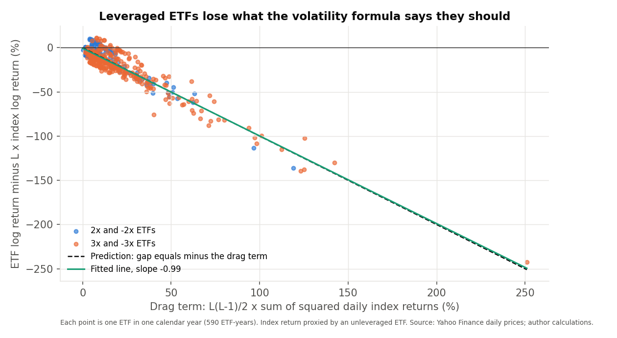
On full calendar years the slope is −0.99 (clustered standard error 0.03, R-squared 0.90), −1.04 for 2× funds and −0.98 for 3× funds. Leveraged and inverse funds both lose to the formula (−0.96 and −1.06), which is why shorting both is attractive. The fitted intercept is −0.69% a year and may reflect financing costs, management fees, tracking differences and other effects the simplified formula does not capture. Correcting the leverage history (energy funds) and the financials index moved the slope from −0.91 to −0.99 on all years; this is a second-order test on calendar years, not a reproduction of the original quarterly experiment.
The strategy: what you collect depends on the reset
| All pairs together | Return, % a year | Volatility, % | Max drawdown, % | Worst day, % |
|---|---|---|---|---|
| Reset daily, no borrow fee | 2.8 | 1.2 | −1.0 | −0.8 |
| Reset monthly, no borrow fee | 7.9 | 12.6 | −14.0 | −9.3 |
| Reset monthly, 3% borrow fee | 4.8 | 12.7 | −14.3 | −9.4 |
| Reset monthly, 5% borrow fee | 2.8 | 12.8 | −22.6 | −9.5 |
| Treasury bill ETF alone | 1.6 | 0.3 | −0.5 | −0.4 |
All 16 pairs together, $1 in each pair when it starts, no rebalancing between pairs. Returns on equity; Treasury bills on the same base for comparison.
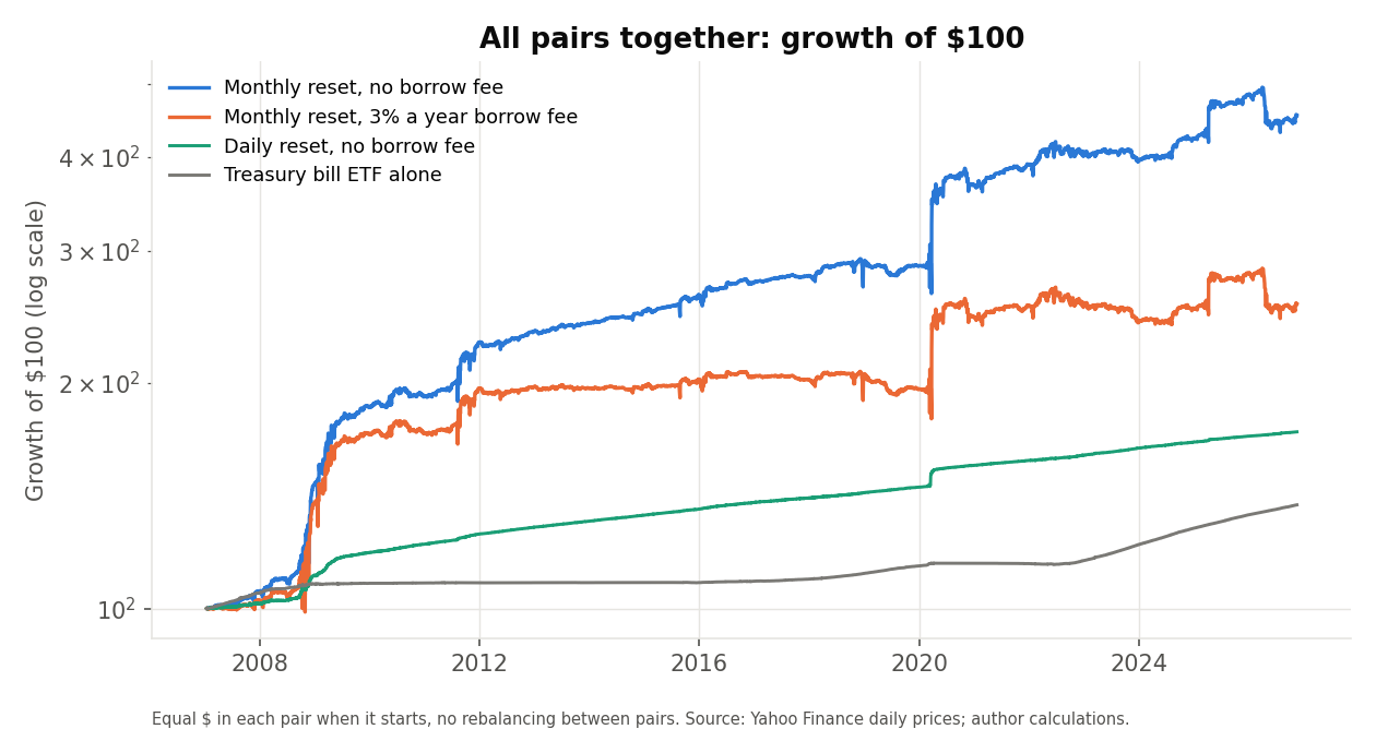
- Daily reset: nothing to collect. The two legs offset each other every day (1.2 points above Treasury bills, about the funds’ fees), so the drag is never collected. A 3% borrow fee takes it below Treasury bills (−0.2%).
- Monthly reset: the drag appears, with 7.9% a year, positive in 16 of 16 pairs, at the cost of 12.6% volatility and a −9.3% worst day. Borrow fees reduce it to 4.8% (3%) and 2.8% (5%), against 1.6% for Treasury bills; the break-even fee is about 6.2%. On the 2010 common period (all pairs trading) the returns are 5.5% and 2.4%, against 1.5% for bills.
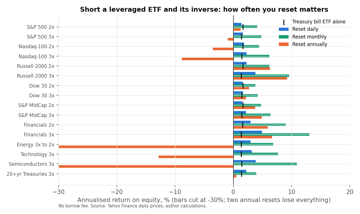
- Annual reset can lose everything: 2 of 16 pairs (energy and semiconductors) were wiped out.
Frictions the idealised model leaves out
| Monthly reset, all pairs | Return, % a year, no borrow fee | Return with 3% borrow fee | Max drawdown, % | Forced liquidations |
|---|---|---|---|---|
| Idealised model | 7.9 | 4.8 | −14.0 | 0 |
| No interest on the short-sale proceeds | 6.3 | 3.2 | −14.2 | 0 |
| 5 bps on each scheduled reset of the shorts | 7.9 | 4.8 | −13.9 | 0 |
| Margin calls (60% or 90% maintenance) | 5.9 | 2.8 | −13.8 | 81 |
| All three together | 4.1 | 1.1 | −14.0 | 81 |
Monthly reset. Margin: if equity falls below the maintenance requirement (60% of the short value for 2× funds, 90% for 3× funds, following FINRA’s rule), the positions are closed that day and the equity waits in cash until the next reset.
- Margin calls matter most. There were 81 forced liquidations across the pairs, and the return falls from 7.9% to 5.9% (2.8% with a 3% borrow fee).
- Interest and trading costs: without interest on the sale proceeds the return is 6.3%; with 5 basis points on each scheduled reset of the short positions it is 7.9%. All three together leave 4.1% before a borrow fee and 1.1% after a 3% fee, against 1.6% for Treasury bills.
Downside risk
The monthly-reset portfolio gained in the 2008–09 crisis (51.5%) and the Covid crash (24.1%), when volatility, and so the drag, was high, but still fell 14.0% from peak to trough in the Covid crash. Single pairs are far riskier: with monthly resets the Energy 3x to 2x pair fell 99% in March 2020, which a margin call would have closed out.
Results for each pair
| Pair | ETFs (long / inverse) | From | Daily reset, % | Monthly reset, % | Monthly, 3% fee, % | Monthly: max drawdown, % | Annual reset, % | T-bill ETF, % |
|---|---|---|---|---|---|---|---|---|
| S&P 500 2x | SSO / SDS | 2007 | 1.4 | 4.1 | 1.0 | −10 | 1.3 | 1.6 |
| S&P 500 3x | UPRO / SPXU | 2009 | 1.6 | 4.8 | 1.7 | −12 | −1.0 | 1.4 |
| Nasdaq-100 2x | QLD / QID | 2007 | 1.8 | 4.5 | 1.4 | −10 | −3.5 | 1.6 |
| Nasdaq-100 3x | TQQQ / SQQQ | 2010 | 2.3 | 6.2 | 3.1 | −11 | −8.9 | 1.4 |
| Russell 2000 2x | UWM / TWM | 2007 | 2.3 | 6.2 | 3.1 | −21 | 6.3 | 1.6 |
| Russell 2000 3x | TNA / TZA | 2008 | 3.8 | 9.6 | 6.4 | −28 | 9.3 | 1.4 |
| Dow 30 2x | DDM / DXD | 2007 | 1.6 | 3.8 | 0.7 | −8 | 2.7 | 1.6 |
| Dow 30 3x | UDOW / SDOW | 2010 | 1.7 | 4.2 | 1.1 | −16 | 2.2 | 1.4 |
| S&P MidCap 2x | MVV / MZZ | 2007 | 1.6 | 4.8 | 1.7 | −20 | 3.7 | 1.6 |
| S&P MidCap 3x | UMDD / SMDD | 2010 | 2.2 | 6.4 | 3.2 | −28 | 4.9 | 1.4 |
| Financials 2x | UYG / SKF | 2007 | 3.0 | 9.0 | 5.8 | −26 | 5.9 | 1.6 |
| Financials 3x | FAS / FAZ | 2008 | 4.9 | 13.0 | 9.7 | −40 | 6.6 | 1.4 |
| Energy 3x to 2x | ERX / ERY | 2008 | 2.9 | 6.8 | 3.7 | −99 | −100.0 | 1.4 |
| Technology 3x | TECL / TECS | 2008 | 3.1 | 7.7 | 4.5 | −23 | −12.8 | 1.4 |
| Semiconductors 3x | SOXL / SOXS | 2010 | 3.8 | 10.9 | 7.6 | −64 | −100.0 | 1.5 |
| 20+yr Treasuries 3x | TMF / TMV | 2009 | 2.2 | 3.9 | 0.9 | −7 | 0.5 | 1.4 |
Annualised return on equity, before borrow fees unless stated. “From” is the first year with data for all four ETFs.
Limitations of this replication
- No original results for the strategy. The book states it without data; the strategy is our own test of its description, and the drag regression is a simplified version of the original.
- Index proxies and benchmark history. Proxies differ from some funds’ actual indexes, and we have not checked every issuer benchmark change.
- Margin and costs. Margin is checked at closing prices with a maintenance requirement only: there is no initial-margin test, no intraday check and no broker-specific rule, so the liquidations are those of our model, not of an actual broker. Trading costs cover only the scheduled resets of the short positions, not the covering of shorts in a liquidation or trades in the Treasury ETF.
- Financing. Borrow fees are scenarios, not data. Whether a broker credits Treasury interest on short-sale proceeds, and the exact margin rules, vary by broker and period; our margin rule is simplified.
- Survivors and overlap. Closed funds are missing, and several pairs share an index, so the pairs are not independent.
- Verification. The R code independently reproduces the regressions and the returns of every pair under every reset, borrow fee and scenario; portfolio aggregation, stress periods and charts are Python only.
Conclusion
The volatility drag of leveraged and inverse ETFs follows the Avellaneda–Zhang formula closely. Whether the book’s strategy collects it depends on the reset: daily resets cancel it, monthly resets earned 7.9% a year before costs. Once margin calls, no interest on the proceeds and trading costs are included, the return falls to 4.1% and, with a 3% borrow fee, 1.1%, against 1.6% for Treasury bills. The drag is a feature of these funds; these simulated returns do not show it could have been captured after all financing, trading and margin constraints.
Code
Each script reads the daily prices, runs the regression and simulates the strategy for every pair, reset, borrow fee and scenario. The shaded block is the strategy simulation. The scripts and results are in the GitHub repository.
"""4.5 Leveraged ETFs: volatility decay of leveraged and inverse ETFs, and the book's strategy of shorting a leveraged ETF together with its
inverse (same leverage, same index) and holding a Treasury bill ETF. Writes data/results_python.json and data/*.csv.
Analysis 1 follows Avellaneda and Zhang (2010): a daily-reset L-times ETF compounds as ln(V_T/V_0) = L ln(S_T/S_0) - L(L-1)/2 * sum(r_u^2) per period.
Leverage history: ERX/ERY were +-3x until 31 Mar 2020 and +-2x after; UYG/SKF tracked the Dow Jones US Financials until 17 Mar 2023 (IYF as proxy), then the
S&P Financial Select Sector index (XLF)."""
import json
from pathlib import Path

import numpy as np
import pandas as pd

ROOT = Path(__file__).resolve().parents[1]
CASH = "SHV"
ERX_CHANGE = pd.Timestamp("2020-04-01")      # first day at +-2x
UYG_CHANGE = pd.Timestamp("2023-03-20")      # first trading day on the S&P Financial Select Sector index
SPEC = {"borrow_pct": [0.0, 1.0, 3.0, 5.0], "rebalance": ["daily", "monthly", "annual"], "min_days_year": 120, "full_year_days": 240, "trade_bps": 5.0,
        "margin_rate": {"2x": 0.6, "3x": 0.9},
        "stress": {"2008-09": ("2008-09-01", "2009-03-31"), "Covid crash 2020": ("2020-02-19", "2020-04-30"), "2022": ("2022-01-01", "2022-12-31")}}
PAIRS = [("S&P 500 2x", "SPY", "SSO", "SDS", 2), ("S&P 500 3x", "SPY", "UPRO", "SPXU", 3), ("Nasdaq-100 2x", "QQQ", "QLD", "QID", 2), ("Nasdaq-100 3x", "QQQ", "TQQQ", "SQQQ", 3),
         ("Russell 2000 2x", "IWM", "UWM", "TWM", 2), ("Russell 2000 3x", "IWM", "TNA", "TZA", 3), ("Dow 30 2x", "DIA", "DDM", "DXD", 2), ("Dow 30 3x", "DIA", "UDOW", "SDOW", 3),
         ("S&P MidCap 2x", "MDY", "MVV", "MZZ", 2), ("S&P MidCap 3x", "MDY", "UMDD", "SMDD", 3), ("Financials 2x", "XLF", "UYG", "SKF", 2), ("Financials 3x", "XLF", "FAS", "FAZ", 3),
         ("Energy 3x to 2x", "XLE", "ERX", "ERY", 3), ("Technology 3x", "XLK", "TECL", "TECS", 3), ("Semiconductors 3x", "SOXX", "SOXL", "SOXS", 3),
         ("20+yr Treasuries 3x", "TLT", "TMF", "TMV", 3)]

px = pd.read_csv(ROOT / "data/prices_all.csv", index_col=0, parse_dates=True, float_precision="round_trip").sort_index()


def pair_frame(p):
    name, u, lp, lm, L = p
    c = [u, lp, lm, CASH] + (["IYF"] if name == "Financials 2x" else [])
    if any(x not in px for x in c):
        return None
    r = px[c].dropna().pct_change().iloc[1:]
    if name == "Financials 2x":                      # Dow Jones US Financials proxy (IYF) before the benchmark change, XLF after
        r[u] = np.where(r.index < UYG_CHANGE, r["IYF"], r[u])
        r = r[[u, lp, lm, CASH]]
    r.columns = ["u", "p", "m", "c"]
    r["L"] = float(L)
    if name.startswith("Energy"):
        r.loc[r.index >= ERX_CHANGE, "L"] = 2.0
    return r


F = {p[0]: pair_frame(p) for p in PAIRS}
F = {k: v for k, v in F.items() if v is not None and len(v) > 500}
meta = {p[0]: {"proxy": p[1], "long": p[2], "inverse": p[3], "L": p[4], "start": str(F[p[0]].index.min().date()), "days": len(F[p[0]])} for p in PAIRS if p[0] in F}
out = {"params": {"spec": SPEC, "pairs": meta, "last_date": str(max(v.index.max() for v in F.values()).date()), "cash": CASH}}

# ---------- 1. volatility decay regression ----------
rows = []
for p in PAIRS:
    if p[0] not in F:
        continue
    f = F[p[0]]
    for leg, sign in (("p", 1), ("m", -1)):
        for y, g in f.groupby(f.index.year):
            if len(g) < SPEC["min_days_year"] or g.L.nunique() > 1:        # a year with a change of leverage (ERX/ERY 2020) is left out
                continue
            lev = sign * float(g.L.iloc[0])
            rows.append({"pair": p[0], "etf": p[2] if leg == "p" else p[3], "L": lev, "year": int(y), "n": len(g),
                         "y": float(np.log1p(g[leg]).sum() - lev * np.log1p(g.u).sum()), "x": float(lev * (lev - 1) / 2 * (g.u ** 2).sum()),
                         "etf_ret": float(np.expm1(np.log1p(g[leg]).sum())), "u_ret": float(np.expm1(np.log1p(g.u).sum()))})
D = pd.DataFrame(rows)
D.to_csv(ROOT / "data/decay_etf_years.csv", index=False)


def ols(y, x, cluster):
    X = np.column_stack([np.ones(len(x)), x])
    b, *_ = np.linalg.lstsq(X, y, rcond=None)
    res = y - X @ b
    n, k = X.shape
    XtXi = np.linalg.inv(X.T @ X)
    se = np.sqrt(np.diag(res @ res / (n - k) * XtXi))
    meat = np.zeros((k, k))
    for g in np.unique(cluster):
        s = X[cluster == g].T @ res[cluster == g]
        meat += np.outer(s, s)
    G = len(np.unique(cluster))
    se_c = np.sqrt(np.diag(XtXi @ meat @ XtXi * G / (G - 1) * (n - 1) / (n - k)))
    return b, se, se_c, float(1 - (res @ res) / ((y - y.mean()) ** 2).sum())


dec = {}
FULL = D[D.n >= SPEC["full_year_days"]]
for label, sub in (("all", D), ("full", FULL), ("long", FULL[FULL.L > 0]), ("inverse", FULL[FULL.L < 0]), ("2x", FULL[FULL.L.abs() == 2]), ("3x", FULL[FULL.L.abs() == 3])):
    b, se, sec, r2 = ols(sub.y.to_numpy(), sub.x.to_numpy(), sub.year.to_numpy())
    dec[label] = {"n": int(len(sub)), "intercept": float(b[0]), "intercept_se": float(se[0]), "slope": float(b[1]), "slope_se": float(se[1]), "slope_se_cluster_year": float(sec[1]),
                  "intercept_se_cluster_year": float(sec[0]), "r2": r2, "n_years": int(sub.year.nunique())}
out["decay_regression"] = dec
out["decay_summary"] = {"n_etf_years_all": int(len(D)), "n_etf_years_full": int(len(FULL))}


# ---------- 2. the book's strategy: short the leveraged ETF and its inverse, hold the Treasury ETF ----------
def sim(f, freq, borrow_pct=0.0, trade_bps=0.0, margin=False, share=1.0):
    """Per $1 of equity at the start of each period: short $0.5 of each leg ($1 gross short), the sale proceeds in the Treasury ETF, $1 of collateral
    earning nothing. Positions reset to target at the first day of each period (daily, monthly or annual); between resets the legs drift.
    borrow_pct: annual fee on the short value, charged daily. trade_bps: cost on the value traded at each reset. share: fraction of the Treasury
    ETF return credited on the proceeds (0 = no interest). margin: maintenance requirement on the short value (0.6 for 2x, 0.9 for 3x); if equity falls
    below it the positions are closed that day and the equity stays in cash until the next reset."""
    key = {"daily": np.arange(len(f)), "monthly": f.index.year * 100 + f.index.month, "annual": f.index.year}[freq]
    p, m, c, Lr = f.p.to_numpy(), f.m.to_numpy(), f.c.to_numpy(), f.L.to_numpy()
    fee, n = borrow_pct / 100 / 252, len(f)
    r, E, prev, a, b, cc, col, closed, dead, liq = np.zeros(n), 1.0, None, 0.0, 0.0, 0.0, 1.0, False, False, 0
    for t in range(n):
        if dead:
            continue
        E_pre = E
        if prev is None or key[t] != prev:                                   # reset to target weights; pay for the trades
            traded = abs(0.5 * E - a) + abs(0.5 * E - b)
            E = E - trade_bps / 1e4 * traded
            a, b, cc, col, closed, prev = 0.5 * E, 0.5 * E, E, E, False, key[t]
        if closed:
            r[t] = E / E_pre - 1
            continue
        fee_t = fee * (a + b)
        a, b, cc, col = a * (1 + p[t]), b * (1 + m[t]), cc * (1 + share * c[t]), col - fee_t
        En = col + cc - a - b
        if En <= 0:
            r[t], dead = -1.0, True
            continue
        if margin and En < (SPEC["margin_rate"]["3x"] if Lr[t] >= 3 else SPEC["margin_rate"]["2x"]) * (a + b):
            col, a, b, cc, closed = En, 0.0, 0.0, 0.0, True                    # forced liquidation at the close
            liq += 1
        r[t], E = En / E_pre - 1, En
    return pd.Series(r, index=f.index), liq


def stats(r):
    r = r.dropna()
    eqc = pd.concat([pd.Series([1.0]), (1 + r.reset_index(drop=True)).cumprod()], ignore_index=True)       # start the curve at 1 so an opening loss counts
    yrs = len(r) / 252
    m = r.groupby(r.index.to_period("M")).apply(lambda x: (1 + x).prod() - 1)
    return {"cagr": float((eqc.iloc[-1] ** (1 / yrs) - 1) * 100) if eqc.iloc[-1] > 0 else -100.0, "vol": float(r.std() * np.sqrt(252) * 100),
            "sharpe": float(r.mean() / r.std() * np.sqrt(252)) if r.std() > 0 else float("nan"), "max_dd": float((eqc / eqc.cummax() - 1).min() * 100),
            "worst_day": float(r.min() * 100), "worst_month": float(m.min() * 100), "best_day": float(r.max() * 100),
            "pct_months_pos": float((m > 0).mean() * 100), "days": int(len(r)), "final": float(eqc.iloc[-1]), "wiped_out": bool((r <= -1.0).any())}


SCEN = {"base": {}, "no_interest": {"share": 0.0}, "trade_cost": {"trade_bps": SPEC["trade_bps"]}, "margin": {"margin": True},
        "all": {"share": 0.0, "trade_bps": SPEC["trade_bps"], "margin": True}}
res, rets = {}, {}
for name, f in F.items():
    res[name] = {}
    for freq in SPEC["rebalance"]:
        for bp in SPEC["borrow_pct"]:
            r_, _ = sim(f, freq, bp)
            res[name][f"{freq}|{bp:g}"] = stats(r_)
            rets[(name, freq, bp)] = r_
    res[name]["scen"] = {}
    for sc, kw in SCEN.items():
        for bp in (0.0, 3.0):
            r_, liq = sim(f, "monthly", bp, **kw)
            res[name]["scen"][f"{sc}|{bp:g}"] = {**stats(r_), "liquidations": liq}
            rets[(name, "monthly", bp, sc)] = r_
    res[name]["cash_only"] = stats(f.c)
out["strategy"] = res
KEYS = ("cagr", "vol", "sharpe", "max_dd", "worst_day", "worst_month", "pct_months_pos")
out["strategy_avg"] = {f"{freq}|{bp:g}": {k: float(np.nanmean([res[n][f"{freq}|{bp:g}"][k] for n in res])) for k in KEYS} for freq in SPEC["rebalance"] for bp in SPEC["borrow_pct"]}
out["strategy_counts"] = {"n_wiped_out_annual_0": int(sum(res[n]["annual|0"]["wiped_out"] for n in res)), "n_wiped_out_monthly_0": int(sum(res[n]["monthly|0"]["wiped_out"] for n in res)),
                          "n_pairs": len(res), "n_positive_daily_0": int(sum(res[n]["daily|0"]["cagr"] > 0 for n in res)), "n_positive_daily_3": int(sum(res[n]["daily|3"]["cagr"] > 0 for n in res)),
                          "cash_cagr": float(np.nanmean([res[n]["cash_only"]["cagr"] for n in res]))}


def combine(R):
    """Portfolio of all pairs with $1 put into each pair when it starts and no rebalancing between pairs; return on total equity."""
    E_prev = (1 + R.fillna(0)).cumprod().shift(1).fillna(1.0).where(R.notna())
    return (R * E_prev).sum(axis=1) / E_prev.sum(axis=1)


def portfolio(freq, bp, sc=None):
    return combine(pd.concat({n: (rets[(n, freq, bp, sc)] if sc else rets[(n, freq, bp)]) for n in F}, axis=1))


port, portm = {}, {}
for bp in SPEC["borrow_pct"]:
    port[bp], portm[bp] = portfolio("daily", bp), portfolio("monthly", bp)
    out.setdefault("portfolio", {})[f"{bp:g}"] = stats(port[bp])
    out.setdefault("portfolio_monthly", {})[f"{bp:g}"] = stats(portm[bp])
cash = combine(pd.concat({n: f.c for n, f in F.items()}, axis=1))
out["portfolio"]["cash"] = stats(cash)
out["portfolio_scen"] = {}
for sc in SCEN:
    for bp in (0.0, 3.0):
        pr = portfolio("monthly", bp, sc)
        out["portfolio_scen"][f"{sc}|{bp:g}"] = {**stats(pr), "liquidations": int(sum(res[n]["scen"][f"{sc}|{bp:g}"]["liquidations"] for n in F))}
start_all = max(f.index.min() for f in F.values())                              # common period: only the dates on which all pairs exist
cp = {f"{bp:g}": stats(portm[bp][start_all:]) for bp in (0.0, 3.0)}
cp["cash"], cp["start"] = stats(cash[start_all:]), str(start_all.date())
out["portfolio_common"] = cp
st = {}
for nm, (a, b) in SPEC["stress"].items():
    st[nm] = {}
    for bp in (0.0, 3.0):
        r = portm[bp][a:b]
        st[nm][f"{bp:g}"] = {"ret": float(((1 + r).prod() - 1) * 100), "worst_day": float(r.min() * 100),
                             "max_dd": float(((1 + r).cumprod() / (1 + r).cumprod().cummax() - 1).min() * 100), "days": int(len(r))}
out["stress_monthly"] = st
out["portfolio_monthly_yearly"] = {f"{bp:g}": {str(y): float(((1 + x).prod() - 1) * 100) for y, x in portm[bp].groupby(portm[bp].index.year)} for bp in (0.0, 3.0)}
pd.DataFrame({f"net_{bp:g}": port[bp] for bp in SPEC["borrow_pct"]}).assign(cash=cash).to_csv(ROOT / "data/portfolio_daily.csv")
pd.DataFrame({f"net_{bp:g}": portm[bp] for bp in SPEC["borrow_pct"]}).to_csv(ROOT / "data/portfolio_monthly_daily.csv")
json.dump(out, open(ROOT / "data/results_python.json", "w"), indent=1, default=str)
print("decay", {k: (round(v["slope"], 3), round(v["slope_se"], 3), round(v["slope_se_cluster_year"], 3), v["n"]) for k, v in dec.items()})
print("portfolio daily", {k: round(v["cagr"], 2) for k, v in out["portfolio"].items()}, "monthly", {k: round(v["cagr"], 2) for k, v in out["portfolio_monthly"].items()})
print("scen", {k: (round(v["cagr"], 2), round(v["max_dd"], 1), v["liquidations"]) for k, v in out["portfolio_scen"].items()})
print("common", {k: (round(v["cagr"], 2) if isinstance(v, dict) else v) for k, v in cp.items()})
# Independent R implementation of the 4.5 leveraged-ETF study (see python/letf.py): the volatility-decay regression (Avellaneda-Zhang) and the
# short-both-legs strategy with a Treasury ETF, simulated day by day from share values, including trading costs, no interest on the proceeds and a
# margin-call rule. Writes data/letf_r_*.csv for verification.
suppressPackageStartupMessages(library(data.table))
px <- fread("data/prices_all.csv"); setnames(px, 1, "Date"); px[, Date := as.Date(Date)]; setorder(px, Date)
ERX_CHANGE <- as.Date("2020-04-01"); UYG_CHANGE <- as.Date("2023-03-20")
pairs <- data.table(name = c("S&P 500 2x","S&P 500 3x","Nasdaq-100 2x","Nasdaq-100 3x","Russell 2000 2x","Russell 2000 3x","Dow 30 2x","Dow 30 3x","S&P MidCap 2x","S&P MidCap 3x","Financials 2x","Financials 3x","Energy 3x to 2x","Technology 3x","Semiconductors 3x","20+yr Treasuries 3x"),
  u = c("SPY","SPY","QQQ","QQQ","IWM","IWM","DIA","DIA","MDY","MDY","XLF","XLF","XLE","XLK","SOXX","TLT"),
  p = c("SSO","UPRO","QLD","TQQQ","UWM","TNA","DDM","UDOW","MVV","UMDD","UYG","FAS","ERX","TECL","SOXL","TMF"),
  m = c("SDS","SPXU","QID","SQQQ","TWM","TZA","DXD","SDOW","MZZ","SMDD","SKF","FAZ","ERY","TECS","SOXS","TMV"),
  L = c(2,3,2,3,2,3,2,3,2,3,2,3,3,3,3,3))
get <- function(i) {
  cols <- c("Date", pairs$u[i], pairs$p[i], pairs$m[i], "SHV"); if (pairs$name[i] == "Financials 2x") cols <- c(cols, "IYF")
  f <- na.omit(px[, ..cols]); n <- nrow(f)
  for (v in setdiff(cols, "Date")) set(f, j = v, value = c(NA, f[[v]][-1] / f[[v]][-n] - 1))
  f <- f[-1]
  u <- f[[pairs$u[i]]]; if (pairs$name[i] == "Financials 2x") u <- ifelse(f$Date < UYG_CHANGE, f$IYF, u)
  g <- data.table(Date = f$Date, u = u, p = f[[pairs$p[i]]], m = f[[pairs$m[i]]], c = f$SHV, L = pairs$L[i])
  if (startsWith(pairs$name[i], "Energy")) g[Date >= ERX_CHANGE, L := 2]
  g
}
F <- lapply(seq_len(nrow(pairs)), get); names(F) <- pairs$name
# decay regression: all calendar years with >=120 days, and full years (>=240 days); years with a change of leverage are left out
rows <- list()
for (i in seq_len(nrow(pairs))) for (leg in c("p", "m")) {
  f <- F[[i]]
  for (y in unique(year(f$Date))) { g <- f[year(Date) == y]; if (nrow(g) < 120 || length(unique(g$L)) > 1) next
    lev <- (if (leg == "p") 1 else -1) * g$L[1]
    rows[[length(rows) + 1]] <- data.table(n = nrow(g), year = y, y = sum(log1p(g[[leg]])) - lev * sum(log1p(g$u)), x = lev * (lev - 1) / 2 * sum(g$u^2)) } }
D <- rbindlist(rows); res <- list()
for (nm in c("all", "full")) { d <- if (nm == "all") D else D[n >= 240]; fit <- lm(y ~ x, d)
  res[[nm]] <- data.table(sample = nm, n = nrow(d), intercept = coef(fit)[1], slope = coef(fit)[2], r2 = summary(fit)$r.squared) }
fwrite(rbindlist(res), "data/letf_r_decay.csv")
# strategy
sim <- function(f, freq, borrow = 0, trade_bps = 0, margin = FALSE, share = 1) {
  per <- switch(freq, daily = seq_len(nrow(f)), monthly = format(f$Date, "%Y-%m"), annual = format(f$Date, "%Y"))
  fee <- borrow / 100 / 252; n <- nrow(f); r <- numeric(n); E <- 1; prevper <- NULL; dead <- FALSE
  a <- 0; b <- 0; cc <- 0; col <- 1; closed <- FALSE
  for (t in seq_len(n)) {
    if (dead) next
    E_pre <- E
    if (is.null(prevper) || per[t] != prevper) {
      traded <- abs(0.5 * E - a) + abs(0.5 * E - b); E <- E - trade_bps / 1e4 * traded
      a <- 0.5 * E; b <- 0.5 * E; cc <- E; col <- E; closed <- FALSE; prevper <- per[t]
    }
    if (closed) { r[t] <- E / E_pre - 1; next }
    fee_t <- fee * (a + b)
    a <- a * (1 + f$p[t]); b <- b * (1 + f$m[t]); cc <- cc * (1 + share * f$c[t]); col <- col - fee_t
    En <- col + cc - a - b
    if (En <= 0) { r[t] <- -1; dead <- TRUE; next }
    if (margin && En < (if (f$L[t] >= 3) 0.9 else 0.6) * (a + b)) { col <- En; a <- 0; b <- 0; cc <- 0; closed <- TRUE }
    r[t] <- En / E_pre - 1; E <- En
  }
  r
}
cagr <- function(r) { fin <- prod(1 + r); if (fin > 0) (fin^(252 / length(r)) - 1) * 100 else -100 }
out <- list()
for (i in seq_len(nrow(pairs))) {
  for (freq in c("daily", "monthly", "annual")) for (bp in c(0, 1, 3, 5))
    out[[length(out) + 1]] <- data.table(pair = pairs$name[i], scen = paste0(freq, "|", bp), cagr = cagr(sim(F[[i]], freq, bp)))
  for (sc in c("base", "no_interest", "trade_cost", "margin", "all")) for (bp in c(0, 3)) {
    a <- list(share = if (sc %in% c("no_interest", "all")) 0 else 1, trade_bps = if (sc %in% c("trade_cost", "all")) 5 else 0, margin = sc %in% c("margin", "all"))
    out[[length(out) + 1]] <- data.table(pair = pairs$name[i], scen = paste0("scen:", sc, "|", bp), cagr = cagr(do.call(sim, c(list(F[[i]], "monthly", bp), a))))
  }
}
fwrite(rbindlist(out), "data/letf_r_strategy.csv"); cat("done\n")
References
Kakushadze, Z. and Serur, J. A. (2018). 151 Trading Strategies. Available at SSRN: https://ssrn.com/abstract=3247865. Source paper
Implemented here: Chapter 4 (Exchange-traded funds), §4.5 “Strategy: Leveraged ETFs (LETFs)”, p. 64–65 and footnote 82.
Avellaneda, M. and Zhang, S. (2010). Path-dependence of leveraged ETF returns. SIAM Journal on Financial Mathematics, 1(1), 586–603. Cited in the book; replicated here
Cheng, M. and Madhavan, A. (2009). The dynamics of leveraged and inverse exchange-traded funds. Journal of Investment Management, 7(4), 43–62. Cited in the book
Data: Yahoo Finance daily prices for the ETFs listed in the repository.