Category: Backtests
Can Donchian Channel Breakouts Beat Buy-and-Hold? A 3-Year QQQ Test
What Did We Test?
This strategy aims to capture price movements by entering long positions when specific conditions, based on recent price action, signal potential upward trends. The approach uses two indicators: the 20-day high, which reflects the highest price over the last 20 days, and two different exponential moving averages (EMAs). The 10-day EMA, which averages prices over ten days while giving more weight to recent prices, must be greater than the 30-day EMA, a longer-term average. This setup suggests that the short-term momentum is stronger than the longer-term trend, potentially indicating a bullish phase.When the conditions for entry are met, the strategy will exit either when the price drops to the 10-day low or when a trailing stop is reached, set at twice the Average True Range (ATR). The ATR is a measure of market volatility, providing a dynamic stop that adjusts based on recent price fluctuations.
What Happened?
The backtest aimed to evaluate a strategy using price indicators to identify potential upward trends in seven symbols from January 1, 2016, to January 1, 2025. Starting with an initial equity of $100,000, the strategy ended with a value of approximately $207,892, resulting in a total return of 107.89%. However, the strategy lagged behind both benchmark comparisons. The equal-weight buy-and-hold basket achieved a total return of 244,286.40%, while the buy-and-hold QQQ index generated a return of 399.43%.One significant caveat of this backtest is that while it generated a positive overall return, the strategy exhibited a maximum drawdown of 25.63%. This decline was notably less severe compared to the 60.66% maximum drawdown of the equal-weight buy-and-hold basket and 35.12% of the QQQ index, indicating better risk management in this regard. Despite this, the strategy’s overall performance did not match the benchmarks, highlighting the importance of evaluating risk alongside return.
How Did It Compare With the Benchmarks?
The strategy executed a total of 152 trades during the backtest period from January 1, 2016, to January 1, 2025. It achieved a total return of 107.89%, which translates to a compounded annual growth rate (CAGR) of 8.47%. However, this performance lagged behind the benchmark of an equal-weight buy-and-hold basket, which returned 244,286.40%, indicating the strategy underperformed by a significant margin.
The Sharpe ratio stands at 1.34, which means that the returns earned were 1.34 times the volatility taken on. In other words, for each unit of risk, the strategy generated a positive return, suggesting a reasonable risk-reward balance. At the trade level, the absence of closed trades listed means that there are no trade details to analyze; thus, it is hard to gauge specific patterns in profitability or consistency.
The monthly returns reveal that the strategy had 22 positive months compared to 13 negative months, indicating a tendency for more frequent gains. The average return during positive months was higher than the average loss during negative months, specifically demonstrating that gains were stronger on average, this pattern aligns with the strategy’s design to capitalize on upward momentum while managing risk through its exit criteria.
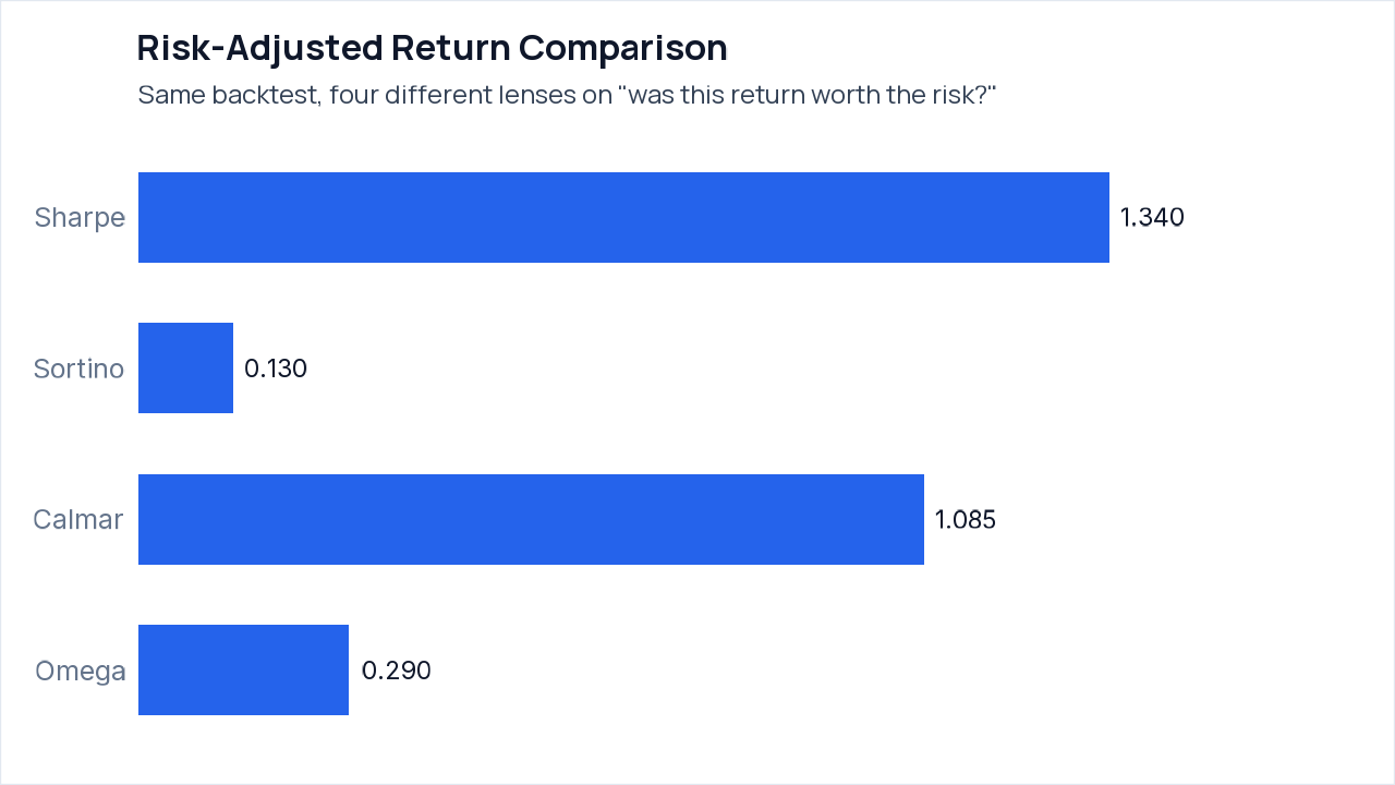
A raw return figure can be misleading because it doesn’t account for the risk taken to achieve those returns. For example, a strategy might return 20% by taking significant risks, but a more modest 10% return could be achieved with much less volatility.
In this backtest, the Sharpe ratio of 1.34 indicates that the strategy generated returns 1.34 times the total volatility, suggesting a reasonable risk-reward balance. The Sortino ratio of 0.13, however, focuses only on downside volatility, revealing that the risk of losing is not well compensated by the upside, which contrasts starkly with the higher Sharpe. The Calmar ratio of 1.08 compares the return to maximum drawdown, further underscoring the strategy’s susceptibility to significant declines.
The "Probability Sharpe > 0" at 99.15% suggests strong statistical confidence that the true Sharpe ratio is positive, which is meaningful. Additionally, since this backtest’s Sharpe ratio is statistically significant, we can trust it provides insightful data. For your own reports, start by comparing the Sharpe and Sortino ratios, followed by the Calmar ratio for a comprehensive risk assessment.
Where Did the Result Come From?
The results of this strategy are concentrated among just a few symbols. The analysis shows that out of the seven symbols traded, only three contributed significantly to the overall profit. Specifically, QQQ led with a net profit of $51,119 from 37 trades and a win rate of 54.1%. MSFT followed with $35,846 from 37 trades and a slightly lower win rate of 45.9%. In contrast, NVDA, while generating a profit of $15,656 from 41 trades, had a win rate of only 29.3%. Other symbols, such as AAPL, had a modest contribution of $6,664 from 37 trades, but there were no trades for XLF, XLP, and XLE.The trade-level significance test indicates that the results should be interpreted with caution. Since there were multiple trades across a few symbols and the p-value reflects the statistical relevance of the results, it is important to note that the nature of overlapping trades means the p-value serves as an indicative measure rather than conclusive evidence.
How Bad Did It Get?
The strategy experienced a maximum drawdown of 25.63%, which means that the account value fell by that percentage from its peak to its lowest point during the backtest. This drawdown lasted for approximately 193 days before hitting the trough and took an additional 60 days to recover. Such statistics indicate that a trader might face considerable losses before seeing their investment recover to previous highs.In terms of risk-adjusted return metrics, the Sharpe ratio is 1.34, suggesting that the returns generated were relatively favorable compared to the level of risk taken. However, the Sortino ratio of 0.13 indicates a substantial disparity between upside potential and downside risk. This divergence highlights a caveat: although the total returns are positive, they may not adequately compensate for the risks involved, especially given that the average drawdown length was 17.82 days. This risk profile should give potential traders pause, as it signals that while profits exist, they come with significant volatility.
The integrity audit failed due to two key issues: first, the trade list did not reconcile with the per-symbol trade statistics, indicating a potential mismatch in reported trades. Second, there was no verification of the gross long exposure relative to the portfolio equity, leaving uncertainty about the strategy’s true risk exposure. These failures suggest that the reported performance might not fully reflect reliable trade execution or risk management.
What Stood Out
- The strategy had a total return of 107.89%, but this was significantly lower than the benchmark’s return of 244,286.40%, highlighting a considerable performance gap.
- Despite a positive monthly return count of 22, the total profit did not keep pace, raising questions about the effectiveness of individual trades contributing to the overall strategy.
- The maximum drawdown of 25.63% indicates notable potential exposure to risk, which could be unexpected given the strategy’s positive return trend.
Limits of This Backtest
- The integrity audit failed, specifically highlighting that the trade list did not reconcile with per-symbol trade statistics, suggesting potential discrepancies in the reported performance.
- There were no closed trade details available, making it difficult to analyze specific performance metrics or patterns.
- The gross long exposure could not be verified relative to portfolio equity, meaning the reported performance may overstate actual returns.
- The total length of the backtest period is 9.00 years, which, while substantial, may not fully capture varying market conditions necessary for a comprehensive evaluation of the strategy.
Monthly Returns
Over the tracking period from January 2023 to January 2025, the strategy experienced a mix of monthly returns, with 22 positive months and 13 negative months. The best month was June 2024, which had a return of 24.48%. Conversely, the worst month was January 2025, with a return of -6.33%.
The most significant drawdown occurred between July 11, 2024, and April 16, 2025, where it reached a depth of -25.63%. This episode aligns with the overall trend of returns, showing that significant declines occurred during a challenging market period.
Conclusions
This backtest revealed a total return of 107.89% over nearly nine years, which amounted to a compounded annual growth rate (CAGR) of 8.47%. However, this performance significantly lagged behind the benchmark of an equal-weight buy-and-hold basket that returned an astonishing 244,286.40%.The primary caveat to consider is the considerable maximum drawdown of 25.63%, which indicates potential for substantial losses during the backtest period. Moreover, the integrity audit highlighted issues, particularly regarding the reconciliation of trade statistics, suggesting that the reported figures may not fully reflect reliable trade execution. Always remember, this walkthrough demonstrates past performance and does not predict future results. If you’re interested, feel free to explore your own strategy ideas using quantstr.at.
Ideas to Test Next
The strategy’s maximum drawdown of 25.63% indicates significant risk exposure, which could make it challenging for traders during downturns. Consider adjusting the exit conditions to include a stop-loss to potentially limit losses and manage risk more effectively.
Enter long when the price breaks above the 20-day high and the 10-day EMA is greater than the 30-day EMA. Exit when the price reaches the 10-day low or hits a trailing stop set at twice the ATR, or if the price falls below a stop-loss of 1.5% from the entry price.
More Backtests
- Can Keltner Channel Breakouts Beat Buy-and-Hold? A 3-Year Test on Tech Equities & QQQ
- MACD SMI Trend Following Across Sector & Global ETFs
- Building and Testing an RSI Mean-Reversion Strategy
Setup, Audit & Replication
Full per-symbol trade statistics ▾
Backtest Integrity Audit: 4 of 6 checks passed
- ✅ Headline Return Matches Ending vs Starting Equity: From dollars: 107.89% | Reported field: 107.89% | Gap: 0.000 pp
- ✅ Equity Curve Starts at Initial Equity and Ends at Ending Value: First point: $100,000 (initial $100,000) | Last point: $207,892 (ending $207,892)
- ✅ Monthly Returns Compound to Headline Return: Compounded months: 107.89% | Headline: 107.89% | Gap: 0.00 pp
- ⚠️ Trade List Reconciles With Per-Symbol Trade Statistics: Trade-list rows: 0 | open at end: 0 | closed per trade statistics: 152 | open rows isolated: yes
- ✅ Sharpe Ratio Consistent With Annualized Return and Volatility: Reported Sharpe: 1.34 | Annualized return / volatility: 1.34
- ⚠️ Gross Long Exposure Never Exceeds Portfolio Equity: No position series in results; cannot verify
Does a Market Trend Filter Beat Buy-and-Hold? An Out-of-Sample Test on 989 Stocks
What Did We Test?
This is a market-timing strategy that uses the S&P 500 index fund, SPY, as a broad market filter. It holds the tested stock when SPY closes above its 100-day simple moving average, or SMA. An SMA is the average closing price over a specified number of trading days, so this rule treats SPY as being in a stronger market condition when its current close is above that average.The strategy does not use a separate stock-level indicator. It assigns 100% of the allotted capital to the stock when the market condition is satisfied, with no leverage, and moves to cash otherwise. The condition is evaluated at each day’s close, with any resulting action taken at the next day’s open.
What Happened?
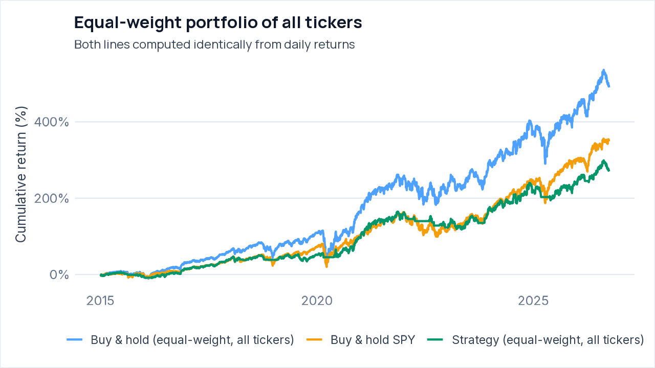
The market-trend filter, which held each stock only while SPY was above its 100-day moving average, beat buy-and-hold by CAGR on 306 of 989 tickers, or 30.9%, during 2015-01-01 to 2026-09-30. The typical result was worse than buy-and-hold, with median excess CAGR of -2.68 percentage points. In the equal-weight portfolio, the strategy had an 11.80% CAGR versus 16.33% for buy-and-hold, while its maximum drawdown was 23.13 percentage points smaller and its Sharpe ratio was higher by 0.05.The main caveat is that the tickers were current S&P 500, S&P 400, and S&P 600 constituents, so companies removed from those indexes during the window are absent, creating survivorship bias. Also, the 989 tickers were not independent: their mean pairwise return correlation was 0.29, and the portfolio excess-return interval ran from -12.42 to 2.67 percentage points, which includes zero.
How Many Tickers Did It Beat Buy-and-Hold On?
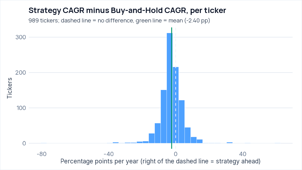
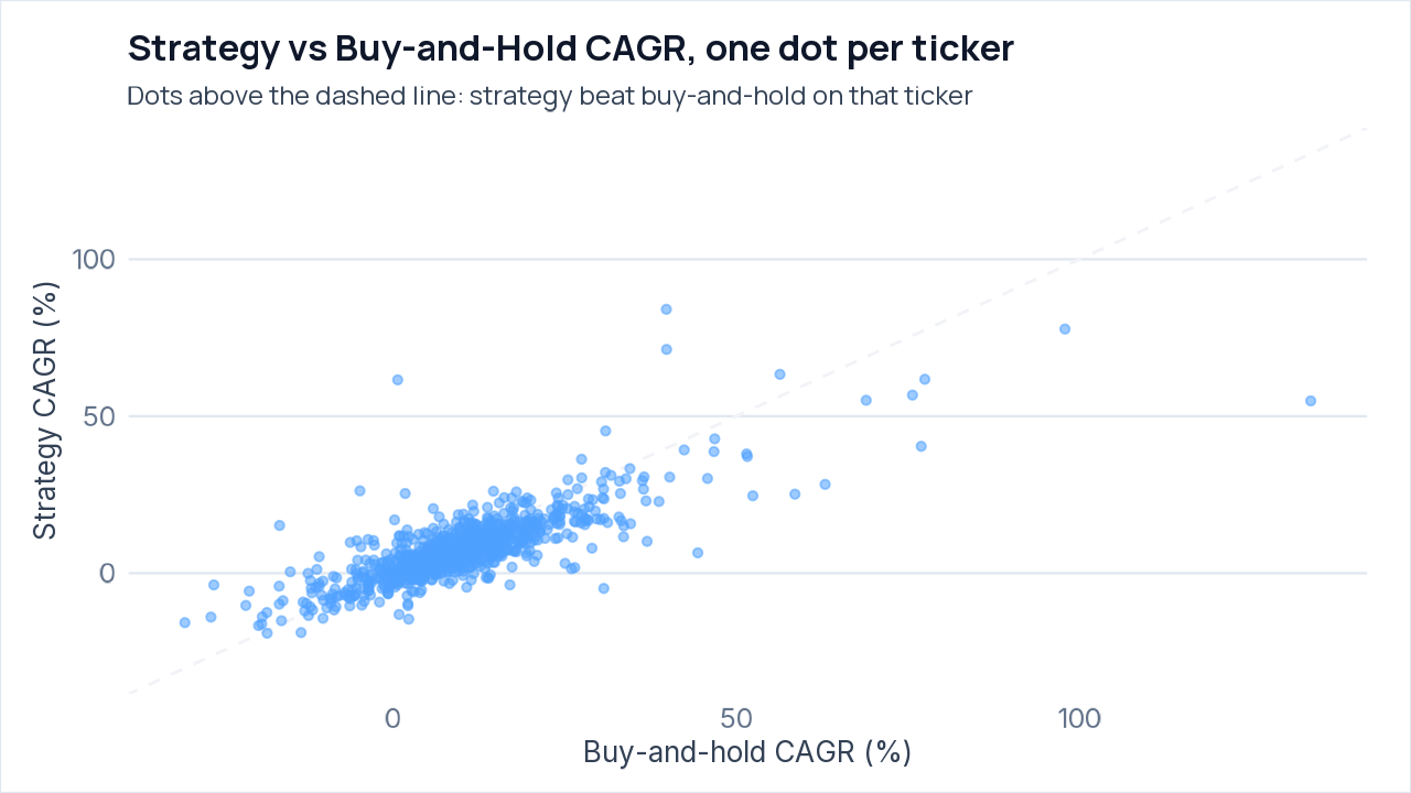
The strategy beat buy-and-hold on an annualized growth rate (CAGR) basis for 306 of 989 tickers, or 30.9%. The excess CAGR versus buy-and-hold had a mean of -2.40 percentage points, a median of -2.68 percentage points, a 10th percentile of -9.15 percentage points, and a 90th percentile of 4.37 percentage points. This means the strategy lagged on most tickers, although the gap was positive for some.
The strategy had a smaller maximum drawdown, the largest decline from a previous peak, on 81.5% of tickers. Median maximum drawdown was 51.83% for the strategy versus 62.86% for buy-and-hold. Its Sharpe ratio, a return measure adjusted for volatility, was better on 32.2% of tickers, with median values of 0.39 versus 0.45, and median time in the market was 79.1%.
Results were consistent in the broad share of winners across the two sub-periods: the strategy beat buy-and-hold on 33.7% of tickers in the first half and 33.5% in the second half. Median excess CAGR remained negative in both, at -22.83 percentage points and -18.64 percentage points. By sector, Communication Services had the highest beat share at 48.5%, followed by Real Estate at 45.3% and Consumer Discretionary at 41.2%; Utilities stood out on the low end at 2.7%, while every sector listed had a negative median excess CAGR.
Is the Result Statistically Significant?
The naive tests point in one direction. The strategy beat buy-and-hold on 306 of 989 tickers, or 30.9%, which is below a 50% coin flip; the exact binomial test gave a p-value of less than 0.0001. A p-value is the probability of seeing a result at least this extreme if there were no real edge. The mean excess CAGR was -2.40 percentage points, with a bootstrap 95% interval of -2.86 to -1.93 percentage points, and the t-test gave t = -10.14 with p = less than 0.0001. On their own, these tests suggest the strategy underperformed buy-and-hold.
Those tests treat the tickers as more independent than they really are. Their mean pairwise correlation was 0.29, making the 989 tickers behave like about 3.5 independent observations; after adjusting for this dependence, the t-statistic was -0.60 and the p-value was 0.5999. That adjusted result is NOT strong evidence of an edge. The equal-weight portfolio comparison also showed lower performance for the strategy, with a CAGR of 11.80% versus 16.33% for buy-and-hold, while the block-bootstrap 95% interval for annualised excess return was -12.42 to 2.67 percentage points, which includes zero and is therefore NOT strong evidence of an edge.
Ticker-level tests found 77 significant tickers at the 5% level, including 76 with a positive mean, while chance alone would produce about 48.6. After the Benjamini-Hochberg false-discovery correction, 0 remained significant, including 0 positive. The pooled-trade test found 50,759 closed trades, a mean return per trade of 2.61%, and p = less than 0.0001, with a 95% interval of 2.42% to 2.80%, but trades overlap in time across tickers, so that p-value is indicative only. The data can show that naive tests and pooled trades look positive in places, but after accounting for ticker dependence and multiple testing, it cannot establish a statistically significant edge over buy-and-hold.
The Equal-Weight Portfolio View
Limits of This Test
What Stood Out
- The strategy portfolio had a lower CAGR than buy-and-hold, 11.80% versus 16.33%, but a smaller maximum drawdown, 17.66% versus 40.79%, and a slightly higher Sharpe ratio, 0.89 versus 0.84.
- The unadjusted excess-CAGR tests had p-values less than 0.0001, but ticker correlation reduced the adjusted result to a t-statistic of -0.60 and a p-value of 0.5999.
- 77 tickers were significant at the 5% level before correction, but 0 remained after Benjamini-Hochberg false-discovery correction.
Limitations
- Survivorship bias applies: Tickers are TODAY’s index members. Companies that were delisted, acquired or removed during the window are absent, which biases buy-and-hold and strategy results upward.
- Tickers are correlated, and each ticker is a standalone backtest rather than a tradable portfolio. The portfolio results therefore do not represent one portfolio holding all positions together under a shared capital allocation.
- The evaluation window may cover a single market regime, so results may not generalize to different market conditions.
- Execution assumes a signal at the close and a fill at the next open, with slippage 5 basis points per fill, no commission, and idle cash earning 0%.
- 11 of 1000 requested tickers were excluded: 1 because the lookback was outside the valid range [1, 66], 1 because it was outside [1, 87], 1 because the series contained non-leading missing values, 5 because they had fewer than 504 bars, and 3 because no price data was returned.
Conclusions
This backtest showed lower returns than buy-and-hold in the equal-weight portfolio, with an 11.80% CAGR versus 16.33%, but a smaller maximum drawdown of 17.66% versus 40.79%. The honest verdict is that it may have reduced drawdowns, but it did not establish a reliable edge over buy-and-hold.The biggest caveat is survivorship bias: the test used current index constituents, so companies removed, acquired, or delisted during the window were absent. This is an educational backtest walkthrough, not investment advice, and past performance in a backtest does not predict future results.
Setup, Audit & Replication
View the exact strategy definition (R) ▾
# =========================================================
# trend_regime_family.R  -- PRE-REGISTERED strategy family (written before any
# results were examined).
#
# One rule family, nine variants: be long a stock while a simple moving-average
# trend condition holds, otherwise sit in cash.
#   filter = "own"    : the stock's close is above its own N-day simple moving average
#   filter = "market" : the market's (SPY) close is above SPY's own N-day moving average
#   filter = "both"   : both conditions hold
#   lookback N in {100, 150, 200} trading days
# Entry when the condition becomes true, exit when it becomes false. Signals are
# evaluated at each bar's close and filled at the next open (engine rule).
# The only free choices are `filter` and `lookback`; they are picked on a
# training set of tickers and an earlier period, then frozen and tested on
# different tickers and a later period (see research_trend_regime.R).
# =========================================================

trend_regime_signals <- function(ohlc, params, market_close) {
  cl <- as.numeric(quantmod::Cl(ohlc))
  n  <- params$lookback
  own_ok    <- cl > TTR::SMA(cl, n)
  market_ok <- market_close > TTR::SMA(market_close, n)
  cond <- switch(params$filter, own = own_ok, market = market_ok, both = own_ok & market_ok)
  list(entry = cond %in% TRUE, exit = (!cond) %in% TRUE)   # NA (insufficient history) -> no action
}

trend_regime_description <- function(filter, lookback) {
  what <- switch(filter,
    own    = sprintf("the stock's closing price is above its own %d-day simple moving average", lookback),
    market = sprintf("the S&P 500 index fund (SPY) closes above its own %d-day simple moving average", lookback),
    both   = sprintf("both the stock's closing price is above its own %d-day simple moving average and SPY closes above its own %d-day simple moving average", lookback, lookback))
  sprintf("Hold the stock (100%% of the capital allotted to it, no leverage) while %s; otherwise hold cash. The condition is checked at each day's close and acted on at the next day's open.", what)
}

make_variant_spec <- function(filter, lookback) {
  list(name = sprintf("Trend filter (%s, %d-day)", filter, lookback),
       description = trend_regime_description(filter, lookback),
       params = list(filter = filter, lookback = lookback),
       needs_market = TRUE,
       signals = trend_regime_signals)
}

trend_regime_variants <- function() {
  g <- expand.grid(filter = c("own", "market", "both"), lookback = c(100, 150, 200), stringsAsFactors = FALSE)
  lapply(seq_len(nrow(g)), function(i) list(id = sprintf("%s_%d", g$filter[i], g$lookback[i]), filter = g$filter[i], lookback = g$lookback[i],
                                            label = sprintf("%s filter, %d-day", c(own = "Own-trend", market = "Market-trend", both = "Own + market trend")[[g$filter[i]]], g$lookback[i])))
}

# FROZEN after selection on training data (see selection.json): filter = "market", lookback = 100
strategy_spec <- make_variant_spec("market", 100)
Integrity Audit: 6 of 6 checks passed
- ✅ Strategy Signals Use Only Past Data: Signals recomputed on truncated history matched the full-history signals at 6 test points.
- ✅ Sample Is Large Enough for Cross-Ticker Statistics: 989 usable tickers (minimum 100)
- ✅ Few Tickers Excluded: 11 of 1000 requested tickers excluded
- ✅ No Ticker Has Missing Headline Metrics: 989 tickers checked
- ✅ Buy-and-Hold Returns Recomputed From Raw Prices Match: REXR: 224.05% vs recorded 224.05% | AXTA: 24.61% vs recorded 24.61% | SONO: 11.51% vs recorded 11.51% | TRST: 136.09% vs recorded 136.09%
- ✅ Independent Cash-Accounting Re-Simulation Matches the Engine: REXR: 215.90% vs recorded 215.90% | AXTA: -14.88% vs recorded -14.88% | SONO: 109.44% vs recorded 109.44% | TRST: 77.85% vs recorded 77.85%
Can Keltner Channel Breakouts Beat Buy-and-Hold? A 3-Year Test on Tech Equities & QQQ
What Did We Test?
This strategy uses a Keltner Channel Volatility Breakout approach, targeting stocks like QQQ, NVDA, AAPL, MSFT, AMD, and AMZN. The Keltner Channel consists of an upper band, a lower band, and a center line, measuring the average price along with average true range (ATR) to capture volatility and identify trends. The Average Directional Index (ADX) is also utilized, which indicates trend strength. Entering long positions when the price breaks above the upper band of the Keltner Channel, combined with an ADX value above 25, suggests a strong upward trend. Exiting positions occurs when the price falls below the center line of the channel.What Happened?
The backtest of the Keltner Channel Volatility Breakout strategy ran from August 29, 2023, to August 27, 2026. The starting capital of $100,000 grew to approximately $207,035, resulting in a total return of 107% and a compound annual growth rate (CAGR) of 27.5%. However, the strategy lagged behind an equal-weight buy-and-hold basket of the same stocks, which achieved a total return of 166% and a CAGR of 38.7%. In contrast, it outperformed the buy-and-hold SPY, which returned 77%.A significant consideration is that the strategy’s results were based on 97 closed trades (+1 still open), which indicates that performance may depend heavily on a limited number of trades. The maximum drawdown for this strategy was approximately 29.9%, compared to the equal-weight benchmark’s max drawdown of 28.9%, suggesting a slightly worse risk profile.
How Did It Compare With the Benchmarks?
The Keltner Channel Volatility Breakout strategy generated a total return of 107% over the 3-year period, resulting in an ending equity value of approximately $207,035 from an initial equity of $100,000. The strategy executed 97 closed trades, with a win rate of about 41%. When compared to the equal-weight buy-and-hold strategy for the same stocks, which achieved a total return of 166%, this strategy lagged significantly by approximately 59%. However, it outperformed the SPY buy-and-hold strategy, which returned 77%, by around 30%.
The Sharpe ratio of 1.12 indicates that the strategy earned 1.12 units of return for every unit of risk taken, which is generally considered acceptable in quantitative trading. At the trade level, the average closed-trade profit and loss was about $1,107. While some trades were profitable, the distribution revealed that a small number of large gains were responsible for a significant portion of the overall profit, indicating a "few big winners" trading pattern.
Monthly returns averaged about 14 positive months versus 20 negative months, with average gains of around 12% during winning months and smaller average losses of about 3%. This suggests that while the strategy struggled to avoid bad months, it was capable of capturing larger upswings, aligning with its volatility breakout approach. However, the strategy faced a maximum drawdown of 30%, indicating considerable risk during its worst performance period.
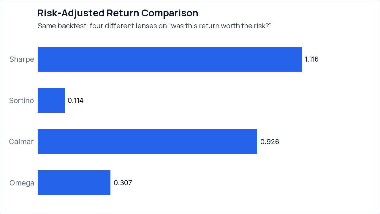
Understanding raw return figures can be misleading, as they fail to reveal the underlying risks involved. For instance, a strategy returning 20% with high volatility may not be preferable to one generating 10% returns with a smoother ride. In this backtest, the Sharpe ratio of 1.12 indicates that the strategy earned about 1.12 units of return per unit of total volatility, reflecting an acceptable risk-return trade-off. The Sortino ratio, at 0.11, looks specifically at downside volatility, signaling concerns since it shows that returns aren’t proportionate to the risks incurred when the strategy performed poorly. The Calmar ratio of 0.93 compares returns relative to the maximum drawdown, offering a different angle that emphasizes the substantial drawdown of nearly 30%.
A key metric, "Probability Sharpe > 0," sits at 97.94%, indicating high confidence that the strategy’s true Sharpe ratio is greater than zero, although the minimum track record needed to ensure this confidence is 487 observations. In this case, the Sharpe ratio is statistically significant, meaning it likely reflects a real pattern rather than being a result of chance. When reviewing your own quantstr.at report, it’s useful to examine the Sharpe and Sortino ratios together to understand risk-adjusted returns, followed by the Calmar ratio for additional insights into maximum drawdown.
Where Did the Result Come From?
The results of this backtest show a significant reliance on a few symbols for the overall performance. While the strategy is built around six symbols, the bulk of the profit is concentrated in just a couple of them. Notably, QQQ accounted for a net profit of $54,264 from 14 trades, translating to a win rate of 57.1% and a profit factor of 8.10. On the other hand, AMZN showed disappointing results, with a net loss of $15,936 across 16 trades, which reflects a win rate of only 25.0% and a low profit factor of 0.21.The significance test indicates that the mean return per trade was 12.22%, with a 95% confidence interval for the mean ranging from -8.03% to 32.46%. The t-statistic was 1.20, and the two-sided p-value was 0.2339, suggesting there isn’t strong evidence that the strategy was definitively effective, primarily due to the small sample size of trades. This means that the returns could be due to random chance rather than a robust underlying strategy.
How Bad Did It Get?
This Keltner Channel Volatility Breakout strategy faces noticeable risks, particularly highlighted by its maximum drawdown of 30%. This means that during its worst period, the strategy could lose close to one-third of its equity before starting to recover. The recovery from this drawdown took about 60 days, indicating significant potential stress over an extended time frame.The risk-adjusted return metrics present a mixed picture. With a Sharpe ratio of 1.12, the strategy earned slightly more than one unit of return for each unit of risk taken, which is generally acceptable. However, the Sortino ratio, at 0.11, indicates that the returns were not proportionate to the downside risk. This suggests that while there were some profitable trades, the good months did not sufficiently outweigh the less favorable ones.
An integrity audit revealed some flaws in the backtesting process, specifically regarding exposure checks. The peak gross long exposure exceeded the actual equity in the account. This means that the reported returns might overstate what a strictly unleveraged account could have achieved. Additionally, the failed percentage checks imply that some of the data’s presentation may lack precision. Hence, while the strategy shows promise, caution is warranted when interpreting its performance metrics due to these inherent risks and issues.
What Stood Out
- The strategy’s total return of 107% significantly lagged behind the equal-weight buy-and-hold benchmark return of 166%, presenting a difference of about 59%.
- Despite a win rate of 41%, the strategy was able to achieve a profit factor of 2.11, indicating that its profitable trades substantially outweighed its losses.
- Some of the most significant gains came from a few standout trades, as excluding the five largest winners resulted in a net loss of about 14%.
Limits of This Backtest
- The strategy generated only 97 closed trades, which may limit statistical significance and overall reliability.
- There was a maximum drawdown of 30%, indicating considerable risk during the worst performance period.
- An integrity audit revealed issues with exposure checks, suggesting that the reported returns could overstate what an unleveraged account could realistically achieve.
- Monthly returns demonstrated more negative months (20) than positive months (14), which indicates more frequent losing periods over the test duration.
Monthly Returns
The backtest reported returns across 37 months, with 14 months showing positive returns, 20 months negative, and 3 months flat. The best month was May 2026, achieving a return of 26%, while the worst was July 2026, with a decline of 7%.
Notably, the largest drawdown episode occurred between July 2024 and April 2025, reaching a depth of 30% over 193 days. This episode aligns with several negative monthly returns, particularly during 2025, which included months of losses.
Conclusions
This backtest of the Keltner Channel Volatility Breakout strategy yielded a total return of 107% over three years, increasing the equity from $100,000 to approximately $207,035. While it did outperform the SPY buy-and-hold strategy, which returned 77%, it lagged significantly behind an equal-weight buy-and-hold basket of the same stocks, which achieved a total return of 166%. The strategy maintained a win rate of about 41% across 97 closed trades, with some large gains contributing disproportionately to the overall profit, implying a reliance on a few big winners.One major caveat to consider is the maximum drawdown of approximately 30%, indicating significant risk during its worst performance phase. This drawdown required about 60 days to recover, highlighting potential stress for traders. It’s important to note that this analysis is purely for educational purposes, not investment advice, and past performance does not guarantee future results. Readers are encouraged to explore their own strategy ideas using quantstr.at.
Ideas to Test Next
The strategy’s maximum drawdown of 30% indicates significant risk during adverse market conditions. By adding a stop-loss, you may help limit losses during downturns, enhancing risk management and potentially improving overall performance.
Trade QQQ, NVDA, AAPL, MSFT, AMD, and AMZN using a Keltner Channel Volatility Breakout strategy. Enter long when price breaks above the 20-period upper band and 14-period ADX > 25 (confirming trend strength). Exit when price closes below the 20-period EMA center line. Additionally, set a stop-loss to exit the position if losses reach 5%.
More Backtests
- MACD SMI Trend Following Across Sector & Global ETFs
- Building and Testing an RSI Mean-Reversion Strategy
- Does a Market Trend Filter Beat Buy-and-Hold? An Out-of-Sample Test on 989 Stocks
Setup, Audit & Replication
Full per-symbol trade statistics ▾
View R Strategy Code ▾
# Load required libraries
library(quantmod)
library(quantstrat)

# Set parameters
start_date <- '2023-08-29'
end_date <- '2026-08-27'
init_equity <- 100000
symbols <- c('QQQ', 'AAPL', 'MSFT', 'NVDA', 'AMD', 'AMZN')

# Get historical data
getSymbols(symbols, from = start_date, to = end_date)

# Initialize the portfolio, account, and orders
initPortf('KeltnerADX', symbols = symbols)
initAcct('KeltnerADX', portfolios = 'KeltnerADX', initEq = init_equity)
initOrders(portfolio = 'KeltnerADX')

# Define the strategy
strategy.st <- 'KeltnerADX'
rm <- 'KeltnerADX'

# Initialize strategy
initStrategy(strategy.st)

# Define indicators
add.indicator(strategy = strategy.st, name = 'EMA', arguments = list(x = quote(Cl(mktdata)), n = 20), label = 'EMA20')
add.indicator(strategy = strategy.st, name = 'KeltnerChannel', arguments = list(HLC = quote(HLC(mktdata)), n = 20, sd = 1.5), label = 'KC')
add.indicator(strategy = strategy.st, name = 'ADX', arguments = list(x = quote(HLC(mktdata)), n = 14), label = 'ADX')

# Define signals
add.signal(strategy = strategy.st, name = 'sigThreshold', arguments = list(column = 'KC.upper', threshold = 0, relationship = 'gt'), label = 'longEntry')
add.signal(strategy = strategy.st, name = 'sigThreshold', arguments = list(column = 'EMA20', threshold = 0, relationship = 'lt'), label = 'longExit')

# Define rules
add.rule(strategy = strategy.st, name = 'ruleSignal', arguments = list(sigcol = 'longEntry', sigval = TRUE, ordertype = 'market', orderside = 'long', replace = FALSE, TxnFees = 0), type = 'enter')
add.rule(strategy = strategy.st, name = 'ruleSignal', arguments = list(sigcol = 'longExit', sigval = TRUE, ordertype = 'market', orderside = 'long', replace = TRUE, TxnFees = 0), type = 'exit')

# Apply the strategy
applyStrategy(strategy = strategy.st, portfolios = 'KeltnerADX')

# Update the portfolio
updatePortf('KeltnerADX')

# Get performance summary
chart.Posn('KeltnerADX', Symbol = 'QQQ')

# Print final portfolio summary
getPortfolio('KeltnerADX')
View Python Strategy Code ▾
import yfinance as yf
import pandas as pd
import vectorbt as vbt

# Set parameters
symbols = ['QQQ', 'AAPL', 'MSFT', 'NVDA']
start_date = '2023-08-29'
end_date = '2026-08-27'

# Download historical data
prices = yf.download(symbols, start=start_date, end=end_date)['Adj Close']

# Calculate indicators
ema20 = prices.ewm(span=20).mean()
upper_band = prices.rolling(window=20).mean() + (prices.rolling(window=20).std() * 1.5)
lower_band = prices.rolling(window=20).mean() - (prices.rolling(window=20).std() * 1.5)
adx = vbt.ADX.run(prices, window=14).adx

# Define entry and exit signals
long_entry = (prices > upper_band) & (adx > 25)
long_exit = prices < ema20

# Create portfolio
portfolio = vbt.Portfolio.from_signals(prices, long_entry, long_exit, init_cash=100000)

# Print portfolio stats
print(portfolio.stats())
View Quarto Markdown Replication (.qmd) ▾
---
title: "Strategy Replication Guide: Keltner ADX Volatility Breakout Strategy"
format: html
editor: visual
execute:
  eval: false
---

# Overview
This Quarto Markdown notebook provides reproducible R and Python code to replicate the **Keltner ADX Volatility Breakout Strategy** backtest (2023-08-29 to 2026-08-27).

## R Replication (quantstrat)

```{r}
#| label: r-strategy-replication
#| message: false
#| warning: false

# Load required libraries
library(quantmod)
library(quantstrat)

# Set parameters
start_date <- '2023-08-29'
end_date <- '2026-08-27'
init_equity <- 100000
symbols <- c('QQQ', 'AAPL', 'MSFT', 'NVDA', 'AMD', 'AMZN')

# Get historical data
getSymbols(symbols, from = start_date, to = end_date)

# Initialize the portfolio, account, and orders
initPortf('KeltnerADX', symbols = symbols)
initAcct('KeltnerADX', portfolios = 'KeltnerADX', initEq = init_equity)
initOrders(portfolio = 'KeltnerADX')

# Define the strategy
strategy.st <- 'KeltnerADX'
rm <- 'KeltnerADX'

# Initialize strategy
initStrategy(strategy.st)

# Define indicators
add.indicator(strategy = strategy.st, name = 'EMA', arguments = list(x = quote(Cl(mktdata)), n = 20), label = 'EMA20')
add.indicator(strategy = strategy.st, name = 'KeltnerChannel', arguments = list(HLC = quote(HLC(mktdata)), n = 20, sd = 1.5), label = 'KC')
add.indicator(strategy = strategy.st, name = 'ADX', arguments = list(x = quote(HLC(mktdata)), n = 14), label = 'ADX')

# Define signals
add.signal(strategy = strategy.st, name = 'sigThreshold', arguments = list(column = 'KC.upper', threshold = 0, relationship = 'gt'), label = 'longEntry')
add.signal(strategy = strategy.st, name = 'sigThreshold', arguments = list(column = 'EMA20', threshold = 0, relationship = 'lt'), label = 'longExit')

# Define rules
add.rule(strategy = strategy.st, name = 'ruleSignal', arguments = list(sigcol = 'longEntry', sigval = TRUE, ordertype = 'market', orderside = 'long', replace = FALSE, TxnFees = 0), type = 'enter')
add.rule(strategy = strategy.st, name = 'ruleSignal', arguments = list(sigcol = 'longExit', sigval = TRUE, ordertype = 'market', orderside = 'long', replace = TRUE, TxnFees = 0), type = 'exit')

# Apply the strategy
applyStrategy(strategy = strategy.st, portfolios = 'KeltnerADX')

# Update the portfolio
updatePortf('KeltnerADX')

# Get performance summary
chart.Posn('KeltnerADX', Symbol = 'QQQ')

# Print final portfolio summary
getPortfolio('KeltnerADX')
```

## Python Replication (VectorBT)

```{python}
#| label: python-strategy-replication

import yfinance as yf
import pandas as pd
import vectorbt as vbt

# Set parameters
symbols = ['QQQ', 'AAPL', 'MSFT', 'NVDA']
start_date = '2023-08-29'
end_date = '2026-08-27'

# Download historical data
prices = yf.download(symbols, start=start_date, end=end_date)['Adj Close']

# Calculate indicators
ema20 = prices.ewm(span=20).mean()
upper_band = prices.rolling(window=20).mean() + (prices.rolling(window=20).std() * 1.5)
lower_band = prices.rolling(window=20).mean() - (prices.rolling(window=20).std() * 1.5)
adx = vbt.ADX.run(prices, window=14).adx

# Define entry and exit signals
long_entry = (prices > upper_band) & (adx > 25)
long_exit = prices < ema20

# Create portfolio
portfolio = vbt.Portfolio.from_signals(prices, long_entry, long_exit, init_cash=100000)

# Print portfolio stats
print(portfolio.stats())
```
Backtest Integrity Audit: 7 of 9 checks passed
- ✅ Headline Return Matches Ending vs Starting Equity: From dollars: 107.03% | Reported field: 107.03% | Gap: 0.000 pp
- ✅ Equity Curve Starts at Initial Equity and Ends at Ending Value: First point: $100,000 (initial $100,000) | Last point: $207,035 (ending $207,035)
- ✅ Monthly Returns Compound to Headline Return: Compounded months: 107.03% | Headline: 107.03% | Gap: 0.00 pp
- ✅ Trade List Reconciles With Per-Symbol Trade Statistics: Trade-list rows: 98 | open at end: 1 | closed per trade statistics: 97 | open rows isolated: yes
- ✅ Sharpe Ratio Consistent With Annualized Return and Volatility: Reported Sharpe: 1.12 | Annualized return / volatility: 1.12
- ⚠️ Gross Long Exposure Never Exceeds Portfolio Equity: Peak gross long exposure was 218.9% of contemporaneous equity (on 2024-08-16)
- ✅ Backtest Generated Closed Trades (>0): Total closed trades executed: 97
- ✅ Reproducible R and Python Code Files Present: strategy_code.R: present | python_vectorbt.py: present
- ⚠️ Prose Percentages Are Integer-Rounded to Whole Numbers: Found unrounded percentages: 29.92%, 13.60%, 681.43%