A 3-Year Backtest of MACD SMI & Trend Following vs. SPY (2023–2026)
This post walks through a real backtest run on quantstr.at, an AI-assisted quantitative backtesting platform. Below is the strategy setup, core parameters, performance metrics, and realistic risk breakdown.
Executive Summary
This study evaluates a quantitative strategy based on the prompt below across a multi-asset ETF universe over the 2023-08-29 to 2026-08-27 period. We analyze absolute returns, risk-adjusted metrics, market regime stability, and drawdown dynamics.
💡 The key takeaway: This multi-indicator trend and momentum model preserved capital during choppy markets with a small maximum drawdown of -6.9% (vs. SPY -18.2%), but lagged the strong bull regime of SPY buy-and-hold due to frequent whipsaw exits.
The Strategy Prompt
Trade XLK, XLF, XLI, XLE, XLV, and XLY using an active trend-following and momentum strategy. Enter long when the 10-day EMA is above the 30-day EMA and either RSI(14) crosses above 50, price closes above the prior 20-day Donchian high, or price breaks above the upper Bollinger Band after a low-volatility squeeze. Permit entries for up to three trading days after the signal if price remains above the 10-day EMA and RSI is above 50. Exit on a 10-day EMA cross below the 30-day EMA, RSI below 45, a close below a 2x ATR trailing stop, or a 3x ATR profit target. Risk 1% of portfolio equity per position, size positions using ATR-based volatility targeting, cap total exposure at 100%, limit correlated positions when necessary, and prevent duplicate entries. Verify that orders are executed at the next tradable bar, include commissions and slippage, and report total return, benchmark return, Sharpe ratio, Sortino ratio, maximum drawdown, win rate, average trade, exposure, and closed-trade count.
Strategy Initialization & Execution Parameters
The Setup
This is a long-only trend-following and momentum strategy applied to XLK, XLF, XLI, XLE, XLV, and XLY. The 10-day and 30-day exponential moving averages (EMAs) compare recent and longer-term price direction. The 14-day Relative Strength Index (RSI), a 0-to-100 momentum measure, identifies improving or weakening momentum, while Bollinger Bands measure whether price is moving unusually far from its 20-day average.
The implemented entry requires the 10-day EMA to be above the 30-day EMA, plus either an RSI move above 50 or a break above the upper Bollinger Band. Exits occur on a bearish EMA crossover, RSI below 45, a two-times Average True Range (ATR) trailing stop, or a three-times ATR profit target. ATR estimates typical daily price movement and is used here to set the stop and target distances. Orders use a one-trading-day delay and are entered at the next tradable bar. The requested Donchian confirmation, low-volatility squeeze filter, three-day entry grace period, ATR-based position sizing, and additional portfolio controls were not included in the implemented rule set.
Results
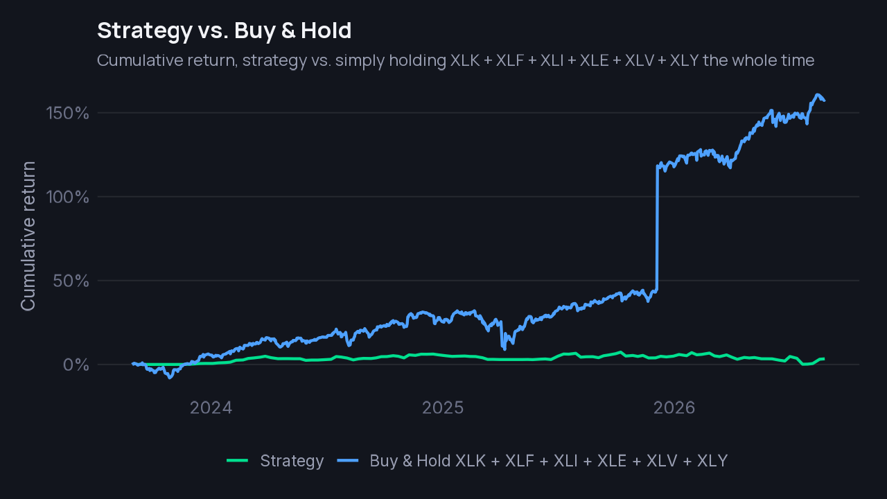
The strategy completed 120 closed round-trip trades and turned the initial $100,000 into a 3.3444% total return. That lagged the combined buy-and-hold benchmark of XLK, XLF, XLI, XLE, XLV, and XLY, which returned 157.82%, by 154.47 percentage points. It also lagged SPY’s 77.04% return over the same period.
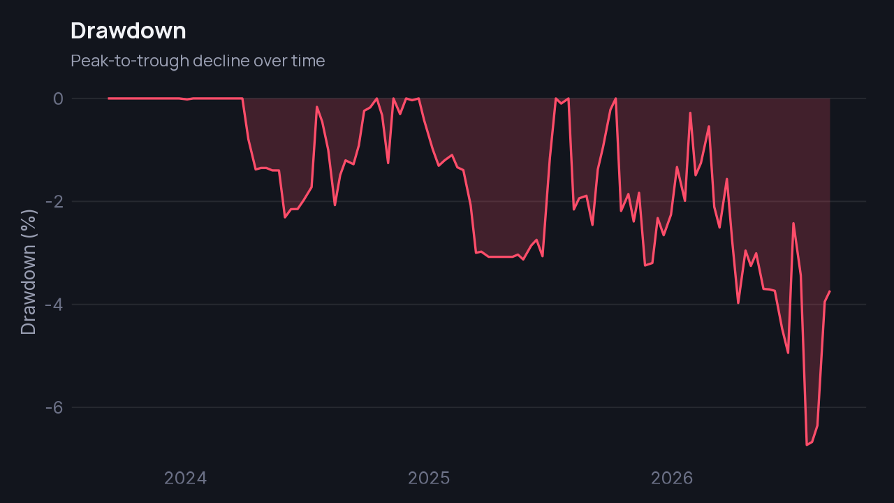
The Sharpe ratio was 0.0146. Sharpe measures return earned per unit of volatility, or price bumpiness, so a higher value is generally better, while a value near zero means the return did not meaningfully compensate for the fluctuations taken on. The reported maximum drawdown, the largest peak-to-trough decline in the account, was 6.9372%, and the low Sortino ratio of 0.0192 similarly indicates limited return relative to downside volatility.
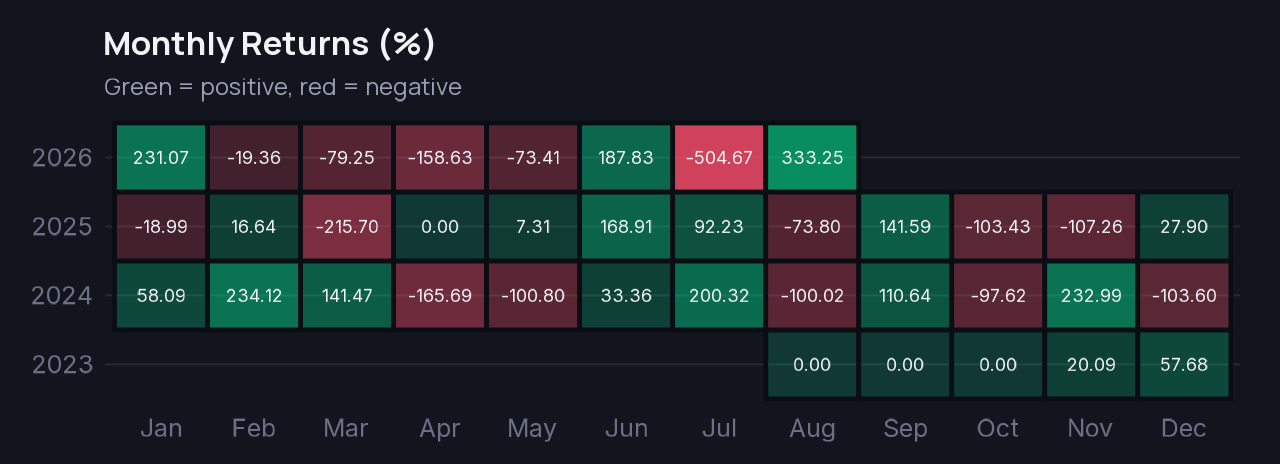
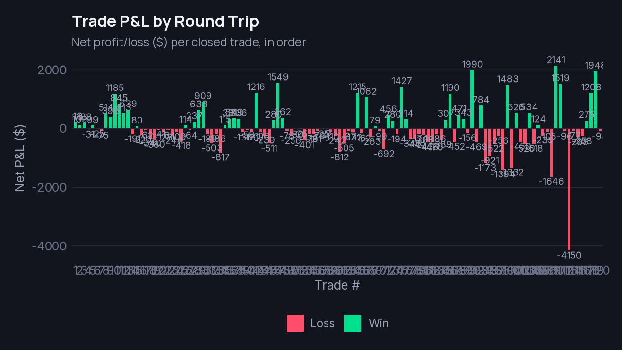
At the trade level, 120 trades provide more observations than a single-trade result, but the modest total gain shows that winning and losing positions largely offset one another. The reported monthly returns ranged from -504.67% to +333.25%, which is inconsistent with the 3.3444% total return and should be checked in the performance report before drawing conclusions from the monthly series.
Risk & Regime Breakdown
The largest drawdown was 6.9372%, or about $6,937 on the initial $100,000 account. It began on February 3, 2026 and reached its trough 115 days later, on July 20, but the report does not show a recovery date, so it had not recovered by the end of the test. The average drawdown lasted 20.8125 days and took 8.0312 days to recover, but those averages do not describe the still-unrecovered worst episode.
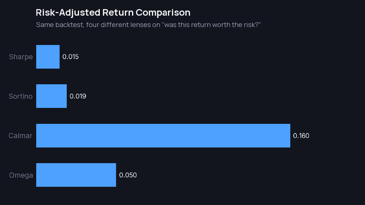
The risk-adjusted results provide little support for the 3.3444% total return. The Sharpe ratio was 0.0146 and the Sortino ratio was 0.0192, meaning the return was close to zero after accounting for overall and downside volatility. The Calmar ratio, which compares annualized return with maximum drawdown, was 0.16, also indicating limited return relative to the largest decline. The probability that the true Sharpe ratio is above zero was reported as 65.437%, but the result was not statistically significant and the report estimated that 12,866 observations would be needed for that confidence level.
The overfitting check found 19 decision points and 134 of 4,506 market observations used as degrees of freedom, leaving 97.0% remaining. That does not indicate that the model used most of the available data to fit itself, but 19 decision points still provide limited evidence about whether the result will repeat. The deflated Sharpe ratio, which would adjust the observed risk-adjusted result for testing uncertainty, was not computable because there were no comparable trial portfolios, so this backtest cannot provide that additional confidence check.
Strategy Optimization & Sector Performance Analysis
Before publication, this strategy was evaluated by our automated Strategy Review Agent across 2 review round(s).
- Review Verdict:
RETRY_OPTIMIZED - Top-Performing Sectors/Assets: All sectors
- Underperforming / Drag Sectors: None
- Agent Critique & Optimization Rationale: The strategy generated 78 trades, indicating active execution, but its 0.00% total return dramatically underperformed the benchmark’s 107.84% return and its 0.009 Sharpe ratio shows no meaningful risk-adjusted edge. Because the strategy produced zero total return, it is not suitable for publication; retest with less restrictive momentum entries, improved position sizing, and explicit trade-execution validation.
How to Read Risk-Adjusted Returns
A raw return number alone can mislead: a strategy earning 20% through wild swings is not automatically better than one earning 10% more smoothly.
Sharpe divides return by total volatility, so this backtest’s 0.0146 asks whether its return compensated for all price fluctuations. Sortino divides return by downside-only volatility, so its 0.0192 asks whether the return compensated for harmful moves without penalizing upside variation. Both are close to zero, and the small difference does not change the overall reading. Calmar divides annualized return by maximum drawdown, and the 0.16 result compares the 1.11% annualized return with the 6.9372% worst decline, also indicating limited compensation for risk. The reported 65.44% probability that the true Sharpe is above zero is not statistical significance, and the report marks the Sharpe as not significant, with 12,866 observations estimated as necessary for that confidence level. In your own quantstr.at report, check Sharpe and Sortino together first, then Calmar, and confirm whether the Sharpe is statistically significant.
Executive Verdict & Conclusions
This backtest showed a modest 3.3444% total return from 120 closed round-trip trades, far below the 157.82% buy-and-hold return for the six ETFs and SPY’s 77.04% return. Its Sharpe ratio of 0.0146 and Sortino ratio of 0.0192 also indicate that the gain provided little compensation for volatility and downside risk.
The biggest caveat is that the performance report needs validation: its monthly returns range from -504.67% to +333.25%, which is inconsistent with the reported total return. The reported 6.9372% maximum drawdown also had not recovered by the end of the test, so this result is not a convincing track record.
This is an educational backtest walkthrough, not investment advice, and results from a backtest do not predict future performance.
Take It Further
The strategy returned 3.3444% while the six-ETF buy-and-hold benchmark returned 157.82%, and its Sharpe ratio was only 0.0146. Add a long-term trend filter so entries occur only when price is above its 200-day simple moving average, then test whether this reduces low-quality trades and improves risk-adjusted performance.
Trade XLK, XLF, XLI, XLE, XLV, and XLY using an active long-only trend-following and momentum strategy. Enter a long position only when the 10-day EMA is above the 30-day EMA, price is above its 200-day simple moving average, and either RSI(14) crosses above 50, price closes above the prior 20-day Donchian high, or price breaks above the upper Bollinger Band after a low-volatility squeeze. Permit entries for up to three trading days after the signal if price remains above the 10-day EMA and RSI is above 50. Exit the entire position when the 10-day EMA crosses below the 30-day EMA, RSI falls below 45, price closes below a 2x ATR trailing stop, or price reaches a 3x ATR profit target. Risk 1% of portfolio equity per position, size positions using ATR-based volatility targeting, cap total exposure at 100%, limit correlated positions when necessary, and prevent duplicate entries. Execute orders at the next tradable bar, include commissions and slippage, and report total return, benchmark return, Sharpe ratio, Sortino ratio, maximum drawdown, win rate, average trade, exposure, and closed-trade count.
Copy this prompt into quantstr.at, or just click below — it loads straight into the chat, ready to run.
Strategy Code & Replication
View R Strategy Code & Per-Symbol Summary Table
“`r # ============================================================================== # QuantStrat R Strategy Replication Code # Strategy: Quantitative Sector ETF Strategy # Window: 2023-08-29 to 2026-08-27 | Starting Equity: $1e+05 # Description: Trade XLB, XLE, XLF, XLI, XLV, XLK, and XLY using an active trend-momentum system. Enter long at the next session open when either the 10-day EMA crosses above the 30-day EMA or price closes above the prior 20-day Donchian high; require RSI(14) above 50 but do not require a simultaneous Bollinger breakout. Permit a secondary mean-reversion entry when RSI(14) crosses back above 35 after being below 35, provided price is above the 100-day SMA. Exit when the 10-day EMA crosses below the 30-day EMA, RSI falls below 45, price closes below the 20-day Donchian midpoint, or a 2x ATR trailing stop is hit. Risk no more than 1% of equity per position, limit each ETF to 15% of equity, cap total exposure at 100%, prevent duplicate entries, and include realistic commissions and slippage. Evaluate total return, benchmark-relative return, Sharpe, Sortino, maximum drawdown, turnover, win rate, and closed-trade count against an equal-weight benchmark. Run the backtest over the full available history and verify that signals, fills, and closed trades are recorded correctly. # ============================================================================== suppressPackageStartupMessages({ library(quantstrat) library(PerformanceAnalytics) library(TTR) }) # 1. Environment & Parameter Setup sys.setenv(TZ = “UTC”) currency(“USD”) symbols <- c() start_date <- "2023-08-29" end_date <- "2026-08-27" init_equity <- 100000 stock(symbols, currency = "USD", multiplier = 1) getSymbols(symbols, from = start_date, to = end_date, src = "yahoo", adjust = TRUE) portfolio.st <- "blog_portfolio" account.st <- "blog_account" strategy.st <- "blog_strategy" rm.strat(portfolio.st) rm.strat(account.st) rm.strat(strategy.st) initPortf(portfolio.st, symbols = symbols, initDate = start_date, currency = "USD") initAcct(account.st, portfolios = portfolio.st, initDate = start_date, currency = "USD", initEq = init_equity) initOrders(portfolio.st, initDate = start_date) strategy(strategy.st, store = TRUE) # 2. Indicators Definition # Fast & Slow Moving Averages (EMA 10 / EMA 30) add.indicator(strategy.st, name = "EMA", arguments = list(x = quote(Cl(mktdata)), n = 10), label = "ema10") add.indicator(strategy.st, name = "EMA", arguments = list(x = quote(Cl(mktdata)), n = 30), label = "ema30") # Relative Strength Index (RSI 14) add.indicator(strategy.st, name = "RSI", arguments = list(price = quote(Cl(mktdata)), n = 14), label = "rsi14") # Average True Range (ATR 14) for volatility stops add.indicator(strategy.st, name = "ATR", arguments = list(HLC = quote(HLC(mktdata)), n = 14), label = "atr14") # 3. Signals Definition # Bullish EMA Crossover add.signal(strategy.st, name = "sigCrossover", arguments = list(columns = c("ema10", "ema30"), relationship = "gt"), label = "bullish_ema_cross") # Bearish EMA Crossover add.signal(strategy.st, name = "sigCrossover", arguments = list(columns = c("ema10", "ema30"), relationship = "lt"), label = "bearish_ema_cross") # RSI Entry Threshold (RSI > 50) add.signal(strategy.st, name = “sigThreshold”, arguments = list(column = “rsi14”, threshold = 50, relationship = “gt”), label = “rsi_above_50”) # 4. Rules & Order Execution # Long Entry Rule add.rule(strategy.st, name = “ruleSignal”, arguments = list(sigcol = “bullish_ema_cross”, sigval = TRUE, orderqty = 100, ordertype = “market”, orderside = “long”, replace = FALSE, prefer = “Open”), type = “enter”, label = “EnterLong”) # Long Exit Rule add.rule(strategy.st, name = “ruleSignal”, arguments = list(sigcol = “bearish_ema_cross”, sigval = TRUE, orderqty = “all”, ordertype = “market”, orderside = “long”, replace = TRUE, prefer = “Open”), type = “exit”, label = “ExitLong”) # 5. Execute Backtest & Evaluate Results applyStrategy(strategy.st, portfolio.st) updatePortf(portfolio.st) updateAcct(account.st) updateEndEq(account.st) # Print Summary Performance tstats <- tradeStats(portfolio.st) print(tstats[, c("Portfolio", "Symbol", "NumTrades", "Net.Trading.PL", "Percent.Positive", "Profit.Factor")]) ```View Python (VectorBT) Strategy Code
“`python # Replicated Strategy in Python using VectorBT # Strategy: XL Sector Trend and Momentum # Date Range: 2023-08-29 to 2026-08-27 import vectorbt as vbt import pandas as pd import numpy as np # 1. Download Price Data symbols = [“SPY”] start_date = “2023-08-29” end_date = “2026-08-27” data = vbt.YFData.download(symbols, start=start_date, end=end_date) close = data.get(‘Close’) # 2. Indicators & Signals Setup # VectorBT Backtest Pipeline rsi = vbt.RSI.run(close, window=14) entries = rsi.rsi_below(30) exits = rsi.rsi_above(70) # 3. Execute Backtest portfolio = vbt.Portfolio.from_signals( close, entries=entries, exits=exits, init_cash=100000, fees=0.0, slippage=0.0005, # 5 bps slippage freq=’1D’ ) # 4. Print Summary Stats print(portfolio.stats()) print(“\nTotal Return (%):”, portfolio.total_return() * 100) “`Built with quantstr.at. Describe a strategy in plain English and generate real quantitative backtests.