Summary
This article implements the rule in Section 4.2 of Kakushadze & Serur (2018), 151 Trading Strategies. It is the sector rotation of Section 4.1, except that funds are ranked by their alpha, the part of their return that three well-known risk factors do not explain, instead of by their past return. The three factors come from the influential three-factor model developed by Eugene Fama and Kenneth French. We apply the rule to the nine original SPDR sector funds from January 2000 to September 2026.
Holding the three funds with the highest alpha returned 7.00% a year. That is less than holding all nine equally (8.70%, charged the same trading costs), less than the S&P 500 (8.24%) and less than the momentum rotation of Section 4.1 run on the same months (8.52%). Its worst fall from a peak was −47.2%, against −49.2% for equal weighting and −39.2% for momentum. The regressions show why this is hard: estimated sector alphas are highly uncertain, and only 1.3% of the one-year estimates we computed were statistically distinguishable from zero. Because Fama and French publish their factors with a delay, we also tested lagged factor data and next-day execution (see the factor availability test below): the six timing variants earned between 6.9% and 9.1% a year, so the size of the shortfall depends on timing, although none beat equal weighting.
Introduction
Sector rotation is the idea of moving money between parts of the stock market, such as technology, energy or health care, towards the ones that look best. Each sector can be bought through a sector ETF, a fund that trades like a share. We use the nine original SPDR sector funds: XLB materials, XLE energy, XLF financials, XLI industrials, XLK technology, XLP consumer staples, XLU utilities, XLV health care and XLY consumer discretionary.
The earlier article in this series ranked the funds by their return over the past year and held the leaders (momentum). One weakness of that rule is that a fund can rank first simply because it carries a lot of market risk in a rising market. The rule in this article tries to fix that. It asks how much a fund earned after accounting for the risks it took, and ranks funds by that excess return, called alpha. For example, a fund that rose 20% in a year when the market rose 13%, and that moves one and a half times as much as the market, has done nothing special; a fund that rose 20% while the market was flat has. More precisely, alpha is the average excess return of a fund that is not explained by its estimated exposure to the market, size and value factors. A positive estimated alpha means the fund earned more than the three-factor model would predict over the estimation period; by itself it is not evidence of a persistent investment advantage.
Fama and French: the model behind the rule
Eugene Fama (University of Chicago, Nobel Prize in Economics 2013) and Kenneth French (Dartmouth) are two of the best-known researchers in finance. In a 1993 paper they showed that much of the difference in returns between diversified stock portfolios can be explained by three things:
- The market (MKT). How much the whole stock market earned above the interest rate on safe short-term Treasury bills. This is the classic risk that all shares share.
- Size (SMB, “small minus big”). Over long periods, shares of small companies have tended to earn more than shares of large companies. SMB is the return of a portfolio of small shares minus that of a portfolio of large shares.
- Value (HML, “high minus low”). Cheap shares, with a high book value relative to their price, have tended to earn more than expensive growth shares. HML is the return of cheap shares minus the return of expensive ones.
Their three-factor model says a fund’s return is explained by how much of each factor it carries, plus a constant. That constant, the regression intercept, is the fund’s alpha: the average return that exposure to the market, size and value does not account for. What is left over on each individual day is called the residual. The paper calls it Jensen’s alpha, after Michael Jensen, who proposed this test of fund managers in 1968. Fama and French publish the factor returns for free, every day since 1926, in the Kenneth French data library. That is the data this article uses.
Data and methodology
What the paper specifies and what we chose
The paper gives one formula, one footnote on how to estimate it and no results. It names no data set, no list of ETFs and no sample period. There is therefore no “original data” to match exactly, and this is one explicit implementation, not a reproduction of published returns. We follow the paper’s three-factor regression specification, with returns in excess of the Treasury-bill rate, and use the one-year daily estimation window suggested in its footnotes. We use the official daily Fama-French three-factor dataset from Kenneth French’s Data Library, a standard source for empirical asset-pricing research. The ETF universe is our assumption, the same nine funds as in the Section 4.1 article, so the two results can be compared directly.
| Element | Paper, §4.2 and footnotes | This article |
|---|---|---|
| Signal | Alpha: the intercept of Eq. (364) | Same |
| Factors | The three Fama-French factors MKT, SMB, HML | Same, from the Kenneth French data library (daily file) |
| Returns | ETF returns in excess of the one-month Treasury-bill rate (fn. 50) | Daily ETF return minus the library’s daily risk-free rate |
| Estimation window | “Typically 1 year” (fn. 77) | 252 trading days (the paper’s one year), re-estimated every month. 126 (half a year) and 504 (two years) are our own additions, in the exploratory grid only |
| Weekly returns | Daily or weekly (fn. 77) | Daily only |
| Holding period | As §4.1: typically 1 to 3 months | 1 month |
| Universe | Sector or industry ETFs, none specified | The nine original Select Sector SPDRs, all trading since Dec 1998 |
| Selection | As §4.1: for example the top decile, optionally shorting the bottom decile | Top 1 of 9 (11%, the closest to a decile) and top 3 of 9 (33%, diversified). Long only |
| Weights | Not specified | Equal weights |
| Trading costs | Not specified | 10 bps per unit traded, on drift-adjusted turnover |
| Execution | As §4.1: right after time t | Idealised: at the month-end close that produced the signal |
| Factor availability | Not specified | The final factor value for day t is used at the close of day t. The library publishes factors with a delay, so a live strategy would need to build them itself. Tested in the factor availability test below |
| Not implemented | R-squared variant with a fourth factor (§4.3) | Separate article. Also no short leg |
Data. Daily closing prices from Yahoo Finance, adjusted for dividends and splits, for the nine ETFs and SPY, together with the daily Fama-French factors, from December 1998 to 30 September 2026, the last day of the factor file. Each month-end, the signal uses the previous 252 trading days, so the first signal is at the end of December 1999 and every result starts in January 2000 and covers 321 months. The strategies and benchmarks in the results table use exactly these months; the sensitivity grid and the factor availability test each use their own common months, stated where they appear. The settings were chosen by us from the paper’s description before running anything, but not independently registered, so we report all 12 variants below. The data was retrieved on 13 November 2026, and the factor file is the library’s 202609 vintage. Both the library and Yahoo can revise their history, so the repository keeps SHA-256 checksums of the exact files used (data/MANIFEST.json). The momentum rotation of §4.1 is rerun on exactly the same months and with the same costs, so its figures differ slightly from the earlier article, which ran one month longer (to October 2026).
Eq. (364): measure alpha
Ri(t) is the daily return of ETF i minus the daily Treasury-bill rate. MKT(t), SMB(t) and HML(t) are the three factor returns that day. β1,i, β2,i and β3,i are the ETF’s loadings on them, αi is its alpha and εi(t) is the part of each day’s return nothing else explains.
At the end of each month we fit this equation to the last 252 days of each ETF’s returns, using ordinary least squares: the line (here a plane) that leaves the smallest squared leftovers. The fitted αi is a daily figure; we multiply it by 252 trading days to quote it per year. Nine ETFs and one regression each gives nine alphas per month, and the rule then behaves exactly like the one in §4.1.
y = d[SECTORS].sub(d["RF"], axis=0)          # excess returns (paper's footnote 50)
A = np.column_stack([np.ones(len(X)), X])
b = np.linalg.solve(A.T @ A, A.T @ y)
alpha[m], tstat[m] = b[0], tt[0]Y <- coredata(d[, SECTORS]) - as.numeric(d$RF) # excess returns (paper's footnote 50)
A[m, ] <- lm.fit(cbind(1, X[s, ]), Y[s, ])$coefficients[1, ]A1: select the funds with the highest alpha
Rank 1 is the highest αi. S(t) is the set of the top N ETFs.
This is the paper’s “same as the sector momentum rotation”, with alpha in place of the past return. With nine ETFs a decile is less than one fund, so we run N = 1 and N = 3. Equations A1 to A4 are our formalisation of the paper’s verbal description.
rank = signal.rank(axis=1, ascending=False, method="first")
w_signal = (rank <= n).astype(float).where(signal.notna())top <- order(signal[m, ], decreasing = TRUE)[1:n]A2: weight them equally
With N = 3, each selected ETF gets one third of the portfolio and the other six get nothing.
The weights add up to 1, so there is no cash and no shorting. N = 9 would hold every fund equally with no rotation; we use that as the benchmark, so it runs through exactly the same code and cost model.
w_signal = w_signal.div(w_signal.sum(axis=1), axis=0) # equal weightw <- rep(0, length(SECTORS)); w[top] <- 1 / nA3 and A4: earn next month’s return, pay costs
ri(t+1) is the ETF’s return over the following month and c = 0.10%. di(t) is last month’s weight after the price moves.
The first term of A3 is the weighted return of the chosen ETFs. The t+1 means we trade at the close of month t and earn month t+1, so a signal never uses the period it is paid on; in the code this is shift(1), and removing it would look into the future. This assumes we can trade at the same close that produced the signal, an idealised close-to-close backtest.
The second term is the trading cost. Weights drift during the month because ETFs move by different amounts, so even keeping the same holdings means trading back to equal weights. A4 gives the drifted weights, and cost is charged on the distance from them to the new targets.
r = sect.pct_change(fill_method=None)                       # month-m return of each ETF
w = w_signal.shift(1)                       # trade at month-end, earn NEXT month
gross = (w * r).sum(axis=1, min_count=1)
drifted = w * (1 + r)                       # last month's weights after the month's price moves
drifted = drifted.div(drifted.sum(axis=1), axis=0)
turnover = (w - drifted.shift(1)).abs().sum(axis=1)   # trades needed to get back to target
net = gross - turnover * cost_bps / 1e4g <- sum(w * r[m + 1, ]) # earned over NEXT month
drifted <- w_prev * (1 + r[m, ]) # last month's weights after the month's price moves
drifted <- drifted / sum(drifted)
tn <- if (m == first) 1 else sum(abs(w - drifted)) # trades needed; first month buys everything
net[m + 1] <- g - tn * cost_bps / 1e4Checks. We wrote the strategy twice, in Python (vectorised pandas and numpy, regressions by the normal equations) and in R (a month-by-month loop, regressions by lm.fit). Each downloads its own prices and its own copy of the factor file. All 321 monthly returns of every series agree to within 1.6×10⁻⁶, all 2898 monthly alphas agree to within 3×10⁻⁸ (a daily figure), and both regression tables, the results table, all 12 sensitivity results (each over the same 309 months) and all six timing variants (each over the same 319 months) match. We also recomputed two cases by hand from the raw prices and factors, using a third tool (the statsmodels regression library) and plain loops: the December 2008 signal (top three XLE, XLU and XLP, alphas equal to the pipeline’s to within 4.36×10⁻¹¹, and a January 2009 return of −3.0524%, identical to the backtest), and the February 2009 turnover of 66.7%: 66.7% from changing holdings and a further 0.08 points from drift.
The regressions
Before looking at the strategy it is worth looking at what Eq. (364) says about the nine funds. The first table fits it once to the whole sample, 6,984 trading days from December 1998 to 30 September 2026. Alpha is shown per year, in percent. A t-statistic is the estimate divided by its uncertainty; beyond about 2 (in either direction, shown in bold) a result is unlikely to be luck. R2 is the share of the fund’s daily ups and downs that the three factors explain. This whole-sample fit is descriptive only: it uses observations that were not available to the early trades, and the strategy never uses it.
| ETF | Alpha (% a year) | t-stat | MKT | SMB | HML | R² |
|---|---|---|---|---|---|---|
| XLB | −0.4 | −0.16 | 0.95 | 0.05 | 0.35 | 0.65 |
| XLE | 1.1 | 0.29 | 0.95 | 0.01 | 0.73 | 0.51 |
| XLF | −4.2 | −1.96 | 1.23 | −0.24 | 0.86 | 0.84 |
| XLI | 0.2 | 0.11 | 0.96 | 0.03 | 0.26 | 0.81 |
| XLK | 2.2 | 1.06 | 1.18 | −0.10 | −0.48 | 0.83 |
| XLP | 1.2 | 0.55 | 0.52 | −0.27 | 0.09 | 0.45 |
| XLU | 1.7 | 0.59 | 0.60 | −0.29 | 0.16 | 0.38 |
| XLV | 2.0 | 0.96 | 0.72 | −0.14 | −0.10 | 0.61 |
| XLY | 0.6 | 0.26 | 1.01 | 0.03 | 0.01 | 0.75 |
Whole-sample fit of Eq. (364) to daily excess returns. MKT, SMB and HML columns are the loadings β1,i, β2,i, β3,i.
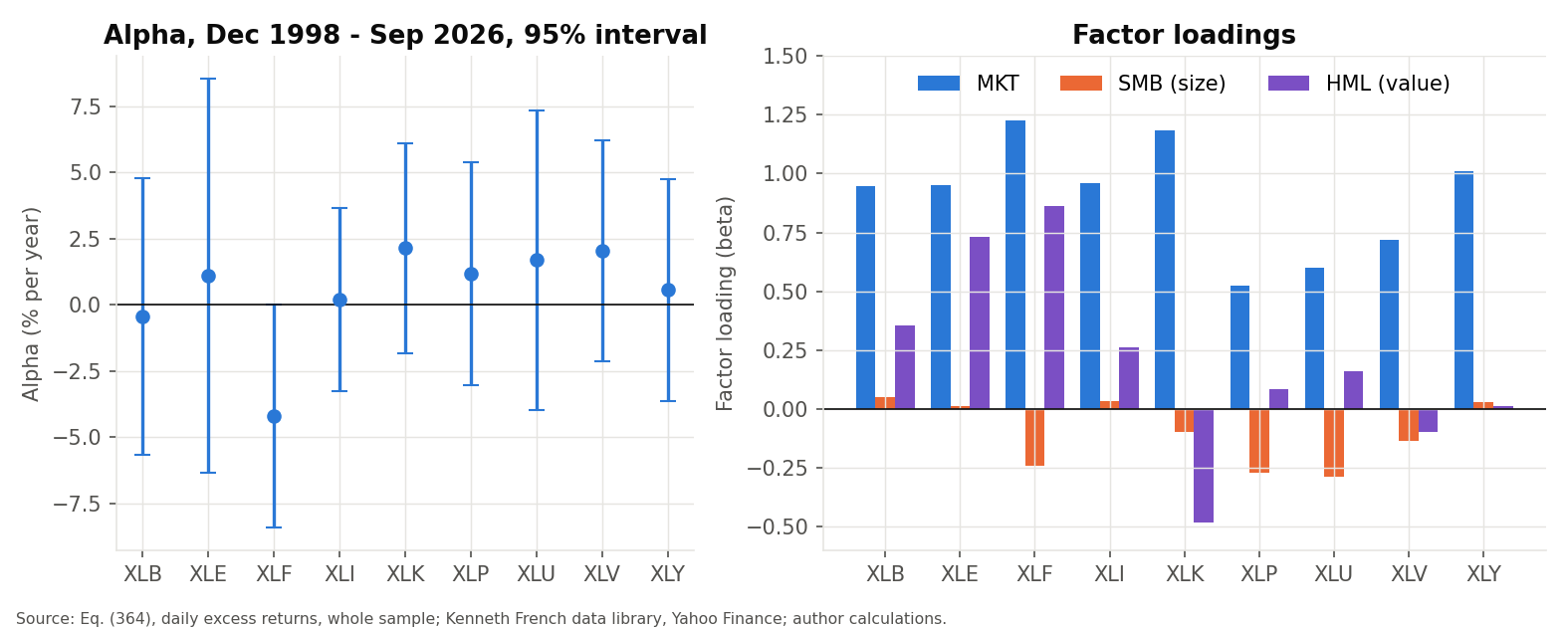
Reading the table. The factors describe the funds sensibly. The market loading is at most 0.72 for XLP, XLU and XLV, the defensive sectors that fall less than the market in a downturn, and at least 1.18 for XLF and XLK, which amplify the market’s moves. The size loading is clearly negative for XLF, XLP and XLU, which hold large, established companies. The value loading is strongly positive for XLE and XLF, whose shares trade cheaply relative to their assets, and negative for XLK, which holds expensive growth shares. The factors explain between 38% of the daily movement (XLU) and 84% (XLF).
The alphas are the point for this strategy, and they are small and uncertain. Over about 28 years, none of the nine is statistically different from zero at the usual 5% level; the strongest case is XLF, at −4.2% a year with a t-statistic of −1.96, just short of the threshold. The standard error of each alpha, even with 6,984 days of data, is between 1.8 and 3.8 percentage points a year. In plain words: once market, size and value exposure is accounted for, the data cannot show that any sector fund has a lasting edge.
The strategy does not use 28 years of data, though. It uses one year, 252 days, which is far less. The second table shows the regression the rule would run at the end of September 2026, ordered by alpha, with the three funds it would buy at the top.
| ETF | Alpha (% a year) | t-stat | MKT | SMB | HML | R² |
|---|---|---|---|---|---|---|
| XLE | 25.9 | 1.27 | 0.00 | −0.18 | 0.69 | 0.14 |
| XLK | 18.5 | 1.38 | 1.63 | −0.43 | −0.36 | 0.75 |
| XLV | 15.7 | 1.04 | 0.29 | 0.43 | 0.21 | 0.13 |
| XLP | −0.6 | −0.04 | 0.03 | 0.36 | 0.40 | 0.13 |
| XLB | −7.0 | −0.53 | 0.88 | 0.35 | 0.63 | 0.46 |
| XLI | −7.3 | −0.63 | 1.02 | 0.18 | 0.40 | 0.56 |
| XLU | −15.4 | −1.04 | 0.24 | 0.15 | 0.35 | 0.08 |
| XLF | −16.1 | −1.46 | 0.78 | 0.12 | 0.54 | 0.46 |
| XLY | −23.8 | −2.01 | 1.11 | 0.24 | 0.04 | 0.64 |
The same regression on the last 252 trading days only. This is the ranking the rule acts on.
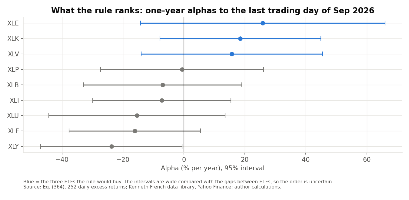
Reading the table. Alphas now run from 25.9% a year for XLE to −23.8% for XLY, which look large. But with one year of data the uncertainty is huge: XLE’s alpha has a t-statistic of only 1.27, and its 95% interval runs from −14% to +66% a year. Only XLY has a t-statistic beyond 2 in either direction. The loadings also shift from year to year: in this window the lowest market loading is 0.00 (XLE), against a whole-sample lowest of 0.52 (XLP). The rule buys XLE, XLK and XLV because they have the highest numbers, but with intervals this wide their order is highly uncertain. Across the whole backtest, the median |t| of a monthly alpha is 0.58 and only 1.3% of the 2898 monthly alphas pass the threshold of 2. Successive one-year windows overlap heavily, so these estimates are not independent observations: the percentage describes how uncertain the estimates are, it is not a formal test. An insignificant alpha is not proof that the true alpha is zero, only that the data gives little evidence for it. The average alpha of the funds the rule picked was 8% a year, measured over the same one-year window the rule looked at; the next sections show what happened afterwards.
Results
| Alpha top 3 | Alpha top 1 | Momentum top 3 (§4.1) | Equal-weight 9 | SPY | |
|---|---|---|---|---|---|
| $100 invested in Jan 2000 became | $611 | $323 | $891 | $931 | $831 |
| CAGR | 7.00% | 4.48% | 8.52% | 8.70% | 8.24% |
| Annual volatility | 15.86% | 21.30% | 14.75% | 14.69% | 15.13% |
| Sharpe ratio (risk-free = 0) | 0.51 | 0.31 | 0.63 | 0.64 | 0.60 |
| Maximum drawdown | −47.2% | −58.1% | −39.2% | −49.2% | −50.8% |
| Months with a gain | 59.5% | 59.2% | 61.1% | 65.1% | 63.2% |
| Average monthly turnover | 47% | 65% | 46% | 3% | 0% |
January 2000 to September 2026. All strategies and the equal-weight portfolio are net of the same 10 bps cost model; the equal-weight portfolio is rebalanced monthly. SPY is buy-and-hold with no trading costs. CAGR is the compound annual growth rate, the Sharpe ratio is return per unit of volatility, and maximum drawdown is the largest fall from a previous peak. Before costs the top-three alpha portfolio earned 7.60% a year (Sharpe 0.54). Its 47% monthly turnover costs 0.56 percentage points a year (turnover × cost × 12); the gap between gross and net CAGR is 0.60, which includes compounding.
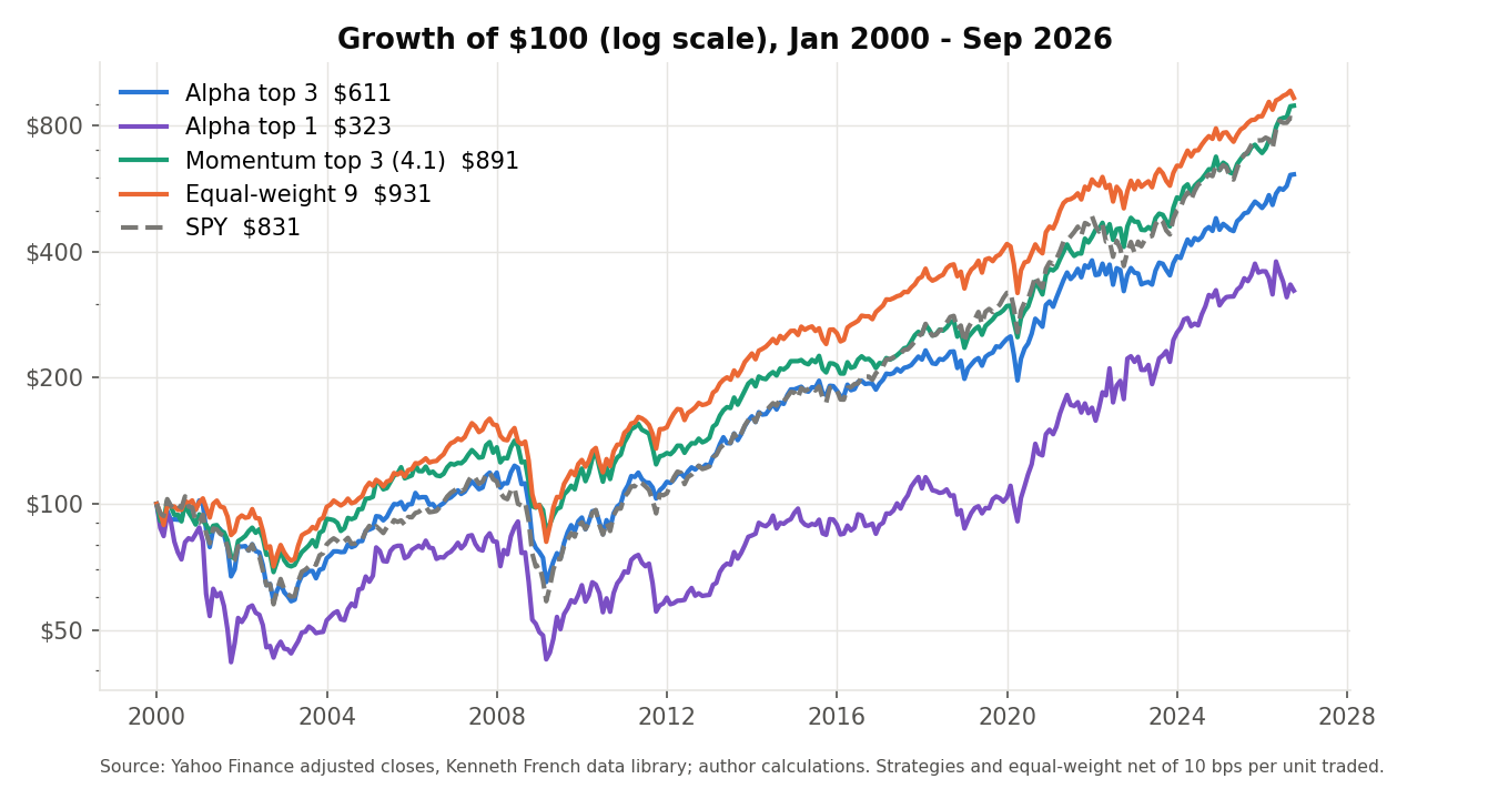
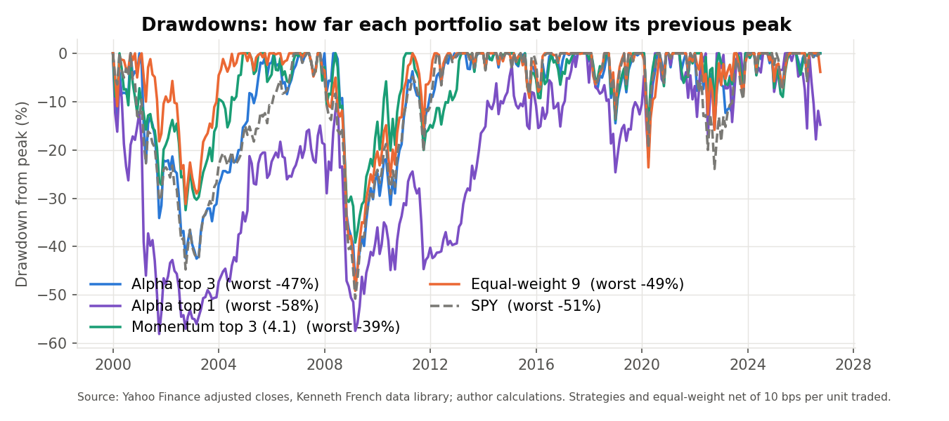
Alpha rotation did not pay. The top-three alpha portfolio earned 7.00% a year, 1.70 percentage points less than equal weighting, with slightly higher volatility (15.9% against 14.7%), and it beat equal weighting in only 12 of 27 calendar years (2026 is January to September). Against the momentum rotation of §4.1 it won 12 of 27 years. The two rules are related but not the same: on average only 2.0 of the three funds they pick coincide in a given month. Concentrating on the single highest alpha was worse still: 4.48% a year, with 21.3% volatility, a 65% monthly turnover and a deepest fall of −58.1%. It did have one good year, 29% in 2022, when energy led.
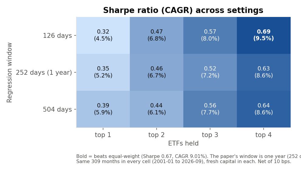
To test whether the settings were unlucky, we re-ran 12 combinations of regression window (126, 252 and 504 trading days) and number of ETFs held (1 to 4). The paper suggests about one year (252 days); 126 and 504 days, half and twice that, are our own experiments. Because a 504-day window needs two years of history before its first alpha, every cell starts with fresh capital in January 2001, the first month all three windows can trade, and covers the same 309 months to September 2026. The equal-weight benchmark is rerun on those months (9.01% a year, Sharpe 0.67). The 252-day top-three cell therefore reads 7.20% a year, not the headline 7.00% over 321 months. These are an exploration of sensitivity, not 12 confirmations of the paper’s strategy. Sharpe ratios range from 0.32 to 0.69. Only 1 setting beats the equal-weight portfolio’s 0.67: the 126-day window with 4 ETFs. The weakest setting earns 4.5% a year. One pattern stands out: the more funds held, the better the result. Averaged over the three windows, CAGR rises from 5.2% for the top one to 8.9% for the top four. That is what we would expect from a signal with little information in it, since holding more funds moves the portfolio towards equal weighting.
Factor availability test
The main result uses each day’s final Fama-French factor values at the close of that same day. The library publishes them later and may revise them, so a live strategy could not have run exactly like this. The paper specifies neither a publication lag nor an execution time, so we leave the main strategy as it is and add a separate test with two changes, applied alone and together. First, the regression window ends 5 or 21 trading days before month-end, a stand-in for the publication delay (21 days is about one monthly update cycle). Second, the trade is made at the next trading day’s close instead of the same close. This is a robustness check, not a reconstruction of what was actually published on each date. Each variant starts with fresh capital in the same month and covers the same 319 months (February 2000 to August 2026): one month later than the main sample, because the lagged window needs a month more history, and one month earlier, because the next-day close after the last month does not exist yet. The two benchmarks are rerun on the same months twice, trading at the month-end close and at the next trading day’s close, so each alpha variant is compared with a benchmark that trades the same way.
| Main (idealised) | Next-day close | 5-day lag | 5-day lag, next-day close | 21-day lag | 21-day lag, next-day close | Equal-weight 9, month-end close | Momentum top 3, month-end close | Equal-weight 9, next-day close | Momentum top 3, next-day close | |
|---|---|---|---|---|---|---|---|---|---|---|
| CAGR | 7.31% | 6.94% | 7.10% | 7.25% | 8.90% | 9.06% | 9.12% | 8.95% | 9.12% | 8.56% |
| Sharpe ratio | 0.53 | 0.49 | 0.51 | 0.51 | 0.63 | 0.62 | 0.67 | 0.66 | 0.63 | 0.63 |
| Maximum drawdown | −47.2% | −50.7% | −48.8% | −49.1% | −47.5% | −49.8% | −49.2% | −39.2% | −51.0% | −42.4% |
| Funds in common with main (of 3) | 3.0 | 3.0 | 2.7 | 2.7 | 2.3 | 2.3 |
February 2000 to August 2026, 319 months, net of 10 bps, fresh capital in each column. “Funds in common” is the average number of the three funds held that are also held by the main version.
No variant beats an equal-weight portfolio that trades the same way (9.12% a year at the month-end close and 9.12% at the next-day close, on these months), so the headline conclusion holds under every timing we tried. But the size of the shortfall depends on timing: 1.8 percentage points a year for the main version, and 0.1 for the closest like-for-like comparison (the 21-day-lag version traded at the next-day close, 9.06% against 9.12%). A one-day execution delay alone moves the CAGR from 7.31% to 6.94%. Delaying the factor data changes which funds are chosen: with a 5-day lag, on average 2.7 of the three funds match the main version’s, and with a 21-day lag 2.3. The 21-day-lag versions did best (8.90% and 9.06%), close to equal weighting and, traded at the next-day close, above momentum (9.06% against 8.56%; at the month-end close momentum earns 8.95%). We do not read that as a better signal: it is the same formula on slightly older data, and a swing this large from shifting the data by a few weeks is consistent with an unstable ranking. The main result is best read as one of several plausible outcomes of the same rule, not as a precise estimate.
Conclusion
Under the implementation choices used in this study, alpha rotation did not outperform an equally weighted portfolio of the nine original Select Sector SPDR ETFs, and in the main version it did not outperform the corresponding sector momentum strategy over the same period. The universe, weighting scheme, rebalancing schedule and transaction costs are our own specification, so these results are one historical implementation of the alpha-ranking framework in Section 4.2, not a reproduction of performance published by the authors. The logic of the idea is sound: a fund’s return should be judged after the market, size and value risks it takes. The difficulty is in the measurement. One year of daily returns is too short to estimate a fund’s alpha precisely, so the alpha ranking is highly uncertain and shifts with small changes in timing, and the portfolio pays about 0.56 points a year in costs for trading on it. Across 12 settings the evidence for an edge is weak, and the settings that come closest to equal weighting do best. The main result also assumes that each day’s final factor values were known at that day’s close. The timing test relaxes this, but it does not reconstruct what was actually published on each date, so this is a historical implementation of the signal, not a fully point-in-time, look-ahead-free implementation.
Limitations. Nine ETFs is a small universe, with few distinct sources of risk for a three-factor model to separate, and it cannot express a true decile. The paper specifies neither data nor sample, so our universe and period are our own choices. The main result is not point-in-time: it uses final factor values for each day at that day’s close, although the library publishes them with a delay and may revise them (see the factor availability test). Execution is idealised: trades happen at the same close that produced the signal. Costs are a flat 10 bps; taxes, wider spreads and market impact are ignored. The strategy is long only, without the paper’s optional short leg, and uses daily rather than weekly returns. Yahoo can revise adjusted prices and the Fama-French library can revise its factors, so rerunning the code later may give slightly different numbers. Past results are not a forecast. The R-squared variant (§4.3) is covered in a separate article.
Code
Each script is self-contained: it downloads the prices and the Fama-French factors, runs the regressions and the strategy, prints both regression tables and the results table and draws the three performance charts shown above. Copy it into a file and run it. Nothing is written to disk. The shaded block is the code behind Eq. (364) and A1 to A4. The results above were produced with Python 3.13.2, pandas 2.3.3, numpy 2.5.3, yfinance 0.2.64; R 4.5.0, quantmod 0.4.28, xts 0.14.1. The monthly returns, weights and alphas behind them are in the GitHub repository.
"""4.2 Strategy: Alpha rotation -- implementation of Kakushadze & Serur (2018),
"151 Trading Strategies", Section 4.2, Eq. (364).

    R_i(t) = alpha_i + b1_i * MKT(t) + b2_i * SMB(t) + b3_i * HML(t) + eps_i(t)

R_i(t) is the ETF's DAILY return in excess of the risk-free rate, and MKT, SMB, HML are the three
Fama-French factors (Kenneth French's data library). The regression uses the last year of daily
returns (252 trading days; the paper's footnote 77: "typically 1 year, daily or weekly returns").
At each month-end: rank the ETFs by alpha_i, buy the top N equal-weighted, hold for one month.
This is the sector momentum rotation of Section 4.1 with the cumulative return replaced by alpha.
"""
import io
import urllib.request
import zipfile

import numpy as np
import pandas as pd
import matplotlib.pyplot as plt
import yfinance as yf   # pip install yfinance

SECTORS = ["XLB", "XLE", "XLF", "XLI", "XLK", "XLP", "XLU", "XLV", "XLY"]
WINDOW = 252        # regression window in trading days (paper: 1 year)
TOP_N = 3           # diversified version; N = 1 is the closest to the paper's top decile
COST_BPS = 10       # cost per unit of turnover, in basis points
T_MOM = 12          # look-back of the Section 4.1 momentum signal used as the comparison
START, END = "1998-12-01", "2026-10-01"   # fixed end date so the sample is reproducible
FF_URL = "https://mba.tuck.dartmouth.edu/pages/faculty/ken.french/ftp/F-F_Research_Data_Factors_daily_CSV.zip"


def download_prices():
    """Daily adjusted closes for the 9 sector ETFs + SPY, straight from Yahoo Finance."""
    tickers = SECTORS + ["SPY"]
    px = yf.download(tickers, start=START, end=END, auto_adjust=True, progress=False)["Close"]
    return px[tickers].dropna(how="all")


def download_factors():
    """Daily Fama-French 3 factors and the risk-free rate (all in percent) from Ken French's library."""
    req = urllib.request.Request(FF_URL, headers={"User-Agent": "Mozilla/5.0"})
    with zipfile.ZipFile(io.BytesIO(urllib.request.urlopen(req).read())) as z:
        lines = z.read(z.namelist()[0]).decode("latin-1").splitlines()
    head = next(i for i, l in enumerate(lines) if l.startswith(",Mkt-RF"))
    rows = []
    for l in lines[head + 1:]:
        p = [x.strip() for x in l.split(",")]
        if len(p) != 5 or not p[0].isdigit():
            break
        rows.append(p)
    ff = pd.DataFrame(rows, columns=["date", "MKT", "SMB", "HML", "RF"]).astype(float)
    ff.index = pd.to_datetime(ff.pop("date").astype(int).astype(str), format="%Y%m%d")
    return ff / 100                              # percent -> decimal


def ff3(y, X):
    """OLS of excess returns y (n x k, one column per ETF) on [1, MKT, SMB, HML] (n x 4).
    Returns coefficients (4 x k: alpha, b_MKT, b_SMB, b_HML), their t-statistics and R-squared."""
    A = np.column_stack([np.ones(len(X)), X])
    b = np.linalg.solve(A.T @ A, A.T @ y)
    e = y - A @ b
    dof = len(A) - A.shape[1]
    se = np.sqrt(np.outer(np.diag(np.linalg.inv(A.T @ A)), (e ** 2).sum(axis=0) / dof))
    r2 = 1 - (e ** 2).sum(axis=0) / ((y - y.mean(axis=0)) ** 2).sum(axis=0)
    return b, b / se, r2


def rolling_alpha(px, ff, window=WINDOW, lag=0):
    """Eq. (364) at each month-end: alpha (and its t-statistic) of every sector ETF over the last
    `window` trading days. Dated by calendar month-end, like the monthly prices.
    lag > 0 is the factor-availability test: the window ends `lag` trading days before month-end,
    as if the factor data were published with that delay (lag = 0 is the main, idealised strategy)."""
    d = pd.concat([px[SECTORS].pct_change(fill_method=None), ff], axis=1, join="inner").dropna()
    y = d[SECTORS].sub(d["RF"], axis=0)          # excess returns (paper's footnote 50)
    X = d[["MKT", "SMB", "HML"]]
    last_day = d.groupby(d.index.to_period("M")).tail(1).index
    alpha, tstat = {}, {}
    for t in last_day:
        i = d.index.get_loc(t) - lag
        if i + 1 < window:
            continue
        s = slice(i + 1 - window, i + 1)
        b, tt, _ = ff3(y.iloc[s].to_numpy(), X.iloc[s].to_numpy())
        m = t + pd.offsets.MonthEnd(0)
        alpha[m], tstat[m] = b[0], tt[0]
    return (pd.DataFrame(alpha, index=SECTORS).T, pd.DataFrame(tstat, index=SECTORS).T)


def to_monthly(px):
    return px.resample("ME").last()             # last trading day of each month


def run(px_m, signal, n=TOP_N, cost_bps=COST_BPS):
    """Same engine as the 4.1 article: `signal` is a month-end score per ETF (higher = better)."""
    sect = px_m[SECTORS]
    r = sect.pct_change(fill_method=None)                       # month-m return of each ETF
    rank = signal.rank(axis=1, ascending=False, method="first")
    w_signal = (rank <= n).astype(float).where(signal.notna())
    w_signal = w_signal.div(w_signal.sum(axis=1), axis=0)   # equal weight
    w = w_signal.shift(1)                       # trade at month-end, earn NEXT month
    gross = (w * r).sum(axis=1, min_count=1)
    drifted = w * (1 + r)                       # last month's weights after the month's price moves
    drifted = drifted.div(drifted.sum(axis=1), axis=0)
    turnover = (w - drifted.shift(1)).abs().sum(axis=1)   # trades needed to get back to target
    first = w.dropna(how="all").index[0]
    turnover.loc[first] = 1.0                   # initial purchase
    net = gross - turnover * cost_bps / 1e4
    out = pd.DataFrame({"gross": gross, "net": net, "turnover": turnover}).loc[first:]
    return out, w.loc[first:]


def from_month(signal, start):
    """Fresh-capital start: ignore the signal before `start`, so the first purchase (and its cost) is at `start`."""
    s = signal.copy()
    s.loc[s.index < start] = np.nan
    return s


def next_close_prices(px):
    """Month-end prices replaced by the close of the NEXT trading day: execution one day after the signal."""
    last = px.groupby(px.index.to_period("M")).tail(1).index
    nxt = px.shift(-1).loc[last]
    nxt.index = nxt.index + pd.offsets.MonthEnd(0)
    return nxt


def stats(ret, label=""):
    ret = ret.dropna()
    yrs = len(ret) / 12
    eq = np.r_[1.0, (1 + ret).cumprod().to_numpy()]      # starts at 1 so an initial loss counts
    dd = eq / np.maximum.accumulate(eq) - 1
    return {
        "label": label,
        "start": str(ret.index[0].date()), "end": str(ret.index[-1].date()),
        "months": int(len(ret)),
        "total_return_pct": round(float(eq[-1] - 1) * 100, 2),
        "cagr_pct": round(float(eq[-1] ** (1 / yrs) - 1) * 100, 2),
        "ann_vol_pct": round(float(ret.std(ddof=1) * np.sqrt(12)) * 100, 2),
        "sharpe": round(float(ret.mean() / ret.std(ddof=1) * np.sqrt(12)), 3),
        "max_drawdown_pct": round(float(dd.min()) * 100, 2),
        "hit_rate_pct": round(float((ret > 0).mean()) * 100, 1),
    }


def regression_table(px, ff, start=None, end=None):
    """Eq. (364) for each ETF over one period: annualised alpha (%), betas, t-statistics, R-squared."""
    d = pd.concat([px[SECTORS].pct_change(fill_method=None), ff], axis=1, join="inner").dropna().loc[start:end]
    b, t, r2 = ff3(d[SECTORS].sub(d["RF"], axis=0).to_numpy(), d[["MKT", "SMB", "HML"]].to_numpy())
    return pd.DataFrame({"alpha_pct_yr": b[0] * 252 * 100, "alpha_t": t[0], "beta_mkt": b[1], "beta_smb": b[2],
                         "beta_hml": b[3], "t_mkt": t[1], "t_smb": t[2], "t_hml": t[3], "r2": r2,
                         "days": len(d)}, index=SECTORS)


def results_table(summary):
    """Net-of-cost results side by side, as a DataFrame."""
    cols = {"Alpha top 3": "alpha3", "Alpha top 1": "alpha1", "Momentum top 3 (4.1)": "mom3",
            "Equal-weight 9 (net)": "equal_weight", "SPY": "spy"}
    return pd.DataFrame({name: {
        "$100 became": 100 * (1 + summary[k]["total_return_pct"] / 100),
        "CAGR (%)": summary[k]["cagr_pct"], "Volatility (%)": summary[k]["ann_vol_pct"],
        "Sharpe": summary[k]["sharpe"], "Max drawdown (%)": summary[k]["max_drawdown_pct"],
        "Months with a gain (%)": summary[k]["hit_rate_pct"],
        "Monthly turnover (%)": summary["avg_monthly_turnover_pct"].get(k, 0.0)}
        for name, k in cols.items()})


def plot_results(series, grid, windows, ns):
    eq = 100 * (1 + pd.DataFrame(series)).cumprod()
    eq = pd.concat([pd.DataFrame(100.0, index=[eq.index[0] - pd.offsets.MonthEnd(1)], columns=eq.columns), eq])  # start at $100
    colors, styles = ["#2a78d6", "#7b4fc4", "#1a9e75", "#eb6834", "grey"], ["-", "-", "-", "-", "--"]
    fig, ax = plt.subplots(3, 1, figsize=(9, 12))
    for c, col, ls in zip(eq.columns, colors, styles):
        ax[0].plot(eq.index, eq[c], color=col, ls=ls, lw=2, label=c)
        ax[1].plot(eq.index, 100 * (eq[c] / eq[c].cummax() - 1), color=col, ls=ls, lw=2)
    ax[0].set_yscale("log"); ax[0].set_title("Growth of $100 (log scale)"); ax[0].legend(frameon=False)
    ax[1].set_title("Drawdown from previous peak (%)")
    sharpe = np.array([[grid[f"W{w}_N{n}"]["sharpe"] for n in ns] for w in windows])
    ax[2].imshow(sharpe, cmap="Blues")
    ax[2].set_xticks(range(len(ns)), ns); ax[2].set_yticks(range(len(windows)), windows)
    ax[2].set_xlabel("ETFs held (n)"); ax[2].set_ylabel("Regression window (trading days)")
    ax[2].set_title("Sharpe ratio by setting (same sample for every cell)")
    for i in range(len(windows)):
        for j in range(len(ns)):
            ax[2].text(j, i, f"{sharpe[i, j]:.2f}", ha="center", va="center")
    fig.tight_layout()
    plt.show()


def main():
    px = download_prices()
    ff = download_factors()
    last = min(px.index[-1], ff.index[-1])      # both series must cover the same last day
    px, ff = px.loc[:last], ff.loc[:last]
    px_m = to_monthly(px)

    alpha, tstat = rolling_alpha(px, ff)        # Eq. (364), one-year daily window
    alpha = alpha.reindex(px_m.index)
    a3, w = run(px_m, alpha)                    # alpha rotation, top 3 of 9
    a1 = run(px_m, alpha, n=1)[0]               # top 1 of 9: closest to the paper's top decile
    mom = px_m[SECTORS] / px_m[SECTORS].shift(T_MOM) - 1     # Section 4.1 signal, Eq. (361)
    idx = a3.index                              # one common sample for everything
    m3 = run(px_m, mom)[0].reindex(idx)         # 4.1 momentum top 3 on the same months
    ew = run(px_m, mom, n=9)[0].reindex(idx)    # all 9 equally, rebalanced monthly, same costs
    spy = px_m["SPY"].pct_change(fill_method=None).loc[idx]

    summary = {
        "params": {"window_days": WINDOW, "top_n": TOP_N, "cost_bps": COST_BPS, "universe": SECTORS,
                   "factors": "Fama-French 3 (daily, Ken French library)", "last_factor_date": str(ff.index[-1].date())},
        "alpha3": stats(a3["net"], "Alpha top 3 of 9 (net)"),
        "alpha3_gross": stats(a3["gross"], "Alpha top 3 of 9 (gross)"),
        "alpha1": stats(a1["net"].reindex(idx), "Alpha top 1 of 9 (net)"),
        "mom3": stats(m3["net"], "Momentum top 3 of 9 (net)"),
        "equal_weight": stats(ew["net"], "Equal-weight 9 (net)"),
        "spy": stats(spy, "SPY buy & hold"),
        "avg_monthly_turnover_pct": {"alpha3": round(float(a3["turnover"].mean()) * 100, 1),
                                     "alpha1": round(float(a1["turnover"].reindex(idx).mean()) * 100, 1),
                                     "mom3": round(float(m3["turnover"].mean()) * 100, 1),
                                     "equal_weight": round(float(ew["turnover"].mean()) * 100, 1)},
    }
    # how alike are the two signals? average overlap of the top-3 sets, and how noisy is alpha?
    top_a = w.loc[idx] > 0
    top_m = (run(px_m, mom)[1].reindex(idx)) > 0
    summary["signal_diagnostics"] = {
        "avg_top3_overlap_with_momentum": round(float((top_a & top_m).sum(axis=1).mean()), 2),
        "pct_alpha_abs_t_above_2": round(float((tstat.reindex(idx).abs() > 2).to_numpy().mean() * 100), 1),
        "median_abs_alpha_t": round(float(tstat.reindex(idx).abs().stack().median()), 2),
        "avg_top3_alpha_pct_yr": round(float((alpha.reindex(idx).where(top_a).stack().mean()) * 252 * 100), 2),
    }
    # exploratory grid: every cell is evaluated on the same months as the main result
    # Every cell, and the equal-weight benchmark, starts with fresh capital in the same month: the first month in
    # which the longest window (504 days) has an alpha. So every cell covers exactly the same months.
    windows, ns, grid = (126, 252, 504), (1, 2, 3, 4), {}
    alphas = {wd: rolling_alpha(px, ff, wd)[0].reindex(px_m.index) for wd in windows}
    g0 = max(a.dropna(how="any").index[0] for a in alphas.values())
    gidx = idx[idx > g0]
    for wd in windows:
        for n in ns:
            s = stats(run(px_m, from_month(alphas[wd], g0), n)[0]["net"].reindex(gidx))
            grid[f"W{wd}_N{n}"] = {"cagr_pct": s["cagr_pct"], "sharpe": s["sharpe"], "months": s["months"]}
    summary["sensitivity"] = grid
    summary["sensitivity_sample"] = {
        "start": str(gidx[0].date()), "end": str(gidx[-1].date()), "months": len(gidx),
        "equal_weight": stats(run(px_m, from_month(mom, g0), n=9)[0]["net"].reindex(gidx), "Equal-weight 9 (net)")}
    # Factor-availability test: alpha from a window that ends `lag` trading days before month-end, and the
    # trade at the same close or at the next trading day's close. Same months and fresh capital for all.
    px_next, variants = next_close_prices(px), {}
    for lag in (0, 5, 21):
        al = rolling_alpha(px, ff, WINDOW, lag)[0].reindex(px_m.index)
        for ex, prices in (("same", px_m), ("next", px_next)):
            variants[(lag, ex)] = (al, prices)
    t0 = max(a.dropna(how="any").index[0] for a, _ in variants.values())
    nets, tops = {}, {}
    for (lag, ex), (al, prices) in variants.items():
        o, wv = run(prices, from_month(al, t0))
        nets[(lag, ex)], tops[(lag, ex)] = o["net"], wv > 0
    tidx = idx[idx > t0]
    for v in nets.values():
        tidx = tidx.intersection(v.dropna().index)
    base = tops[(0, "same")].reindex(tidx)
    summary["timing_test"] = {"start": str(tidx[0].date()), "end": str(tidx[-1].date()), "months": len(tidx), "variants": {
        f"lag{lag}_{ex}": {**stats(nets[(lag, ex)].reindex(tidx)),
                           "top3_overlap_with_main": round(float((tops[(lag, ex)].reindex(tidx) & base).sum(axis=1).mean()), 2)}
        for (lag, ex) in nets},
        "equal_weight": stats(run(px_m, from_month(mom, t0), n=9)[0]["net"].reindex(tidx), "Equal-weight 9 (net)"),
        "mom3": stats(run(px_m, from_month(mom, t0))[0]["net"].reindex(tidx), "Momentum top 3 (net)"),
        # the same two benchmarks traded at the next trading day's close, to compare like with like with the "next" variants
        "equal_weight_next": stats(run(px_next, from_month(mom, t0), n=9)[0]["net"].reindex(tidx), "Equal-weight 9, next-day close (net)"),
        "mom3_next": stats(run(px_next, from_month(mom, t0))[0]["net"].reindex(tidx), "Momentum top 3, next-day close (net)")}
    # calendar-year returns
    yr = pd.DataFrame({"alpha3": a3["net"], "alpha1": a1["net"].reindex(idx), "mom3": m3["net"],
                       "equal_weight": ew["net"], "spy": spy})
    summary["annual_returns_pct"] = (
        ((1 + yr).groupby(yr.index.year).prod() - 1) * 100).round(2).to_dict("index")
    # the regressions themselves: whole sample, and the latest one-year window (what the rule sees today)
    full = regression_table(px, ff)
    latest = regression_table(px, ff, start=px.index[-WINDOW:][0])
    summary["regression_full"] = full.round(4).to_dict("index")
    summary["regression_latest"] = latest.round(4).to_dict("index")

    # ---- SAVE-BEGIN: optional, uncomment to write the results to ./data ----
    # import json
    # from pathlib import Path
    # out = Path("data"); out.mkdir(exist_ok=True)
    # px.to_csv(out / "prices_python.csv"); ff.to_csv(out / "factors_python.csv")
    # (out / "results_python.json").write_text(json.dumps(summary, indent=2, default=str))
    # pd.DataFrame({"alpha3_net": a3["net"], "alpha3_gross": a3["gross"], "alpha1_net": a1["net"].reindex(idx),
    #               "mom3_net": m3["net"], "ew_net": ew["net"], "spy": spy, "turnover_alpha3": a3["turnover"]}
    #              ).to_csv(out / "monthly_returns_python.csv", float_format="%.10f")
    # w.to_csv(out / "weights_python.csv", float_format="%.6f")
    # alpha.to_csv(out / "alphas_python.csv", float_format="%.10f")
    # tstat.to_csv(out / "alpha_tstats_python.csv", float_format="%.6f")
    # full.to_csv(out / "regression_full_python.csv", float_format="%.6f")
    # latest.to_csv(out / "regression_latest_python.csv", float_format="%.6f")
    # ---- SAVE-END ----

    print("Eq. (364) over the whole sample, daily excess returns (alpha in % per year):")
    print(full.round(2).to_string())
    print("\nEq. (364) over the latest one-year window:")
    print(latest.round(2).to_string())
    print("\n" + results_table(summary).round(2).to_string())
    tt = summary["timing_test"]
    print(f"\nFactor-availability test, {tt['start']} to {tt['end']} ({tt['months']} months):")
    print(pd.DataFrame({k: {"CAGR (%)": v["cagr_pct"], "Sharpe": v["sharpe"], "Max drawdown (%)": v["max_drawdown_pct"],
                            "Top-3 overlap with main": v["top3_overlap_with_main"]} for k, v in tt["variants"].items()}).to_string())
    plot_results({"Alpha top 3": a3["net"], "Alpha top 1": a1["net"].reindex(idx), "Momentum top 3 (4.1)": m3["net"],
                  "Equal-weight 9 (net)": ew["net"], "SPY": spy}, grid, windows, ns)
    return a3, w, alpha, px_m, ew, spy, summary


if __name__ == "__main__":
    main()
# 4.2 Strategy: Alpha rotation -- implementation of Kakushadze & Serur (2018),
# "151 Trading Strategies", Section 4.2, Eq. (364):
#     R_i(t) = alpha_i + b1_i * MKT(t) + b2_i * SMB(t) + b3_i * HML(t) + eps_i(t)
# R_i(t) is the ETF's DAILY return in excess of the risk-free rate, and MKT, SMB, HML are the three
# Fama-French factors (Kenneth French's data library). The regression uses the last year of daily
# returns (252 trading days; the paper's footnote 77: "typically 1 year, daily or weekly returns").
# At each month-end: rank the ETFs by alpha_i, buy the top N equal-weighted, hold for one month.
# This is the sector momentum rotation of Section 4.1 with the cumulative return replaced by alpha.
suppressPackageStartupMessages({ library(quantmod); library(xts) })
# install.packages(c("quantmod", "xts"))   # once

SECTORS <- c("XLB","XLE","XLF","XLI","XLK","XLP","XLU","XLV","XLY")
WINDOW <- 252; TOP_N <- 3; COST_BPS <- 10; T_MOM <- 12
START <- "1998-12-01"; END <- "2026-10-01"     # fixed end date (exclusive, as in the Python script) so the sample is reproducible
FF_URL <- "https://mba.tuck.dartmouth.edu/pages/faculty/ken.french/ftp/F-F_Research_Data_Factors_daily_CSV.zip"

# Daily adjusted closes for the 9 sector ETFs + SPY, straight from Yahoo Finance
TICKERS <- c(SECTORS, "SPY")
px <- do.call(merge, lapply(TICKERS, function(s)
  Ad(getSymbols(s, src = "yahoo", from = START, to = END, auto.assign = FALSE))))
colnames(px) <- TICKERS

# Daily Fama-French 3 factors and the risk-free rate (percent) from Ken French's library
zf <- tempfile(fileext = ".zip"); download.file(FF_URL, zf, mode = "wb", quiet = TRUE)
lines <- readLines(unz(zf, "F-F_Research_Data_Factors_daily.csv"), warn = FALSE)
head_i <- grep("^,Mkt-RF", lines)[1]
body <- lines[(head_i + 1):length(lines)]
body <- body[grepl("^[0-9]{8},", body)]                       # data rows only (drops the copyright line)
ff <- read.csv(text = body, header = FALSE, col.names = c("date", "MKT", "SMB", "HML", "RF"))
ff <- xts(ff[, -1] / 100, as.Date(as.character(ff$date), "%Y%m%d"))   # percent -> decimal
last_day <- min(index(px)[nrow(px)], index(ff)[nrow(ff)])             # both series must cover the same last day
px <- px[paste0("/", last_day)]; ff <- ff[paste0("/", last_day)]

pm <- apply.monthly(px, function(x) tail(x, 1))        # month-end prices
index(pm) <- as.Date(format(index(pm), "%Y-%m-01"))    # label by month
months <- format(index(pm), "%Y-%m")

# Daily returns of the ETFs and the factors on common dates
rets <- px[, SECTORS] / lag(px[, SECTORS], 1) - 1
d <- na.omit(merge(rets, ff, join = "inner"))
Y <- coredata(d[, SECTORS]) - as.numeric(d$RF)         # excess returns (paper's footnote 50)
X <- coredata(d[, c("MKT", "SMB", "HML")])
month_end_rows <- tapply(seq_len(nrow(d)), format(index(d), "%Y-%m"), max)

# Eq. (364) at each month-end: alpha of every ETF over the last `window` trading days.
# lag > 0 is the factor-availability test: the window ends `lag` trading days before month-end, as if the
# factor data were published with that delay (lag = 0 is the main, idealised strategy).
rolling_alpha <- function(window = WINDOW, lag = 0) {
  A <- matrix(NA_real_, length(months), length(SECTORS), dimnames = list(months, SECTORS))
  for (m in names(month_end_rows)) {
    i <- month_end_rows[[m]] - lag
    if (i < window) next
    s <- (i - window + 1):i
    A[m, ] <- lm.fit(cbind(1, X[s, ]), Y[s, ])$coefficients[1, ]
  }
  A
}

# Eq. (364) for each ETF over one period, with lm(): annualised alpha (%), betas, t-statistics, R-squared
regression_table <- function(rows) {
  do.call(rbind, lapply(SECTORS, function(s) {
    f <- lm(Y[rows, s] ~ X[rows, ]); cf <- coef(summary(f))
    data.frame(alpha_pct_yr = cf[1, 1] * 252 * 100, alpha_t = cf[1, 3], beta_mkt = cf[2, 1], beta_smb = cf[3, 1],
               beta_hml = cf[4, 1], t_mkt = cf[2, 3], t_smb = cf[3, 3], t_hml = cf[4, 3],
               r2 = summary(f)$r.squared, days = length(rows), row.names = s)
  }))
}

# signal: matrix of month-end scores (months x ETFs); higher = better. Same engine as the 4.1 article.
run_strategy <- function(pm, signal, n = TOP_N, cost_bps = COST_BPS) {
  P <- coredata(pm[, SECTORS]); N <- nrow(P)
  r <- rbind(NA, P[-1, ] / P[-N, ] - 1)                # monthly returns
  first <- which(rowSums(!is.na(signal)) == length(SECTORS))[1]
  w_prev <- rep(0, length(SECTORS))                    # weights held during month m
  gross <- net <- turn <- rep(NA_real_, N)
  for (m in first:(N - 1)) {                           # signal at end of month m
    top <- order(signal[m, ], decreasing = TRUE)[1:n]
    w <- rep(0, length(SECTORS)); w[top] <- 1 / n
    g <- sum(w * r[m + 1, ])                           # earned over NEXT month
    drifted <- w_prev * (1 + r[m, ])                   # last month's weights after the month's price moves
    drifted <- drifted / sum(drifted)
    tn <- if (m == first) 1 else sum(abs(w - drifted)) # trades needed; first month buys everything
    gross[m + 1] <- g
    net[m + 1] <- g - tn * cost_bps / 1e4
    turn[m + 1] <- tn
    w_prev <- w
  }
  data.frame(month = months, gross = gross, net = net, turnover = turn)
}

stats <- function(ret, label) {
  ret <- ret[!is.na(ret)]; yrs <- length(ret) / 12
  eq <- c(1, cumprod(1 + ret)); dd <- eq / cummax(eq) - 1   # starts at 1 so an initial loss counts
  list(label = label, months = length(ret),
       total_return_pct = round((tail(eq, 1) - 1) * 100, 2),
       cagr_pct = round((tail(eq, 1)^(1 / yrs) - 1) * 100, 2),
       ann_vol_pct = round(sd(ret) * sqrt(12) * 100, 2),
       sharpe = round(mean(ret) / sd(ret) * sqrt(12), 3),
       max_drawdown_pct = round(min(dd) * 100, 2),
       hit_rate_pct = round(mean(ret > 0) * 100, 1))
}

alpha <- rolling_alpha()                                                  # Eq. (364), one-year daily window
mom <- coredata(pm[, SECTORS]); mom <- rbind(matrix(NA, T_MOM, length(SECTORS)),
         mom[-(1:T_MOM), ] / mom[1:(nrow(mom) - T_MOM), ] - 1)             # Section 4.1 signal, Eq. (361)
a3  <- run_strategy(pm, alpha)                 # alpha rotation, top 3 of 9
a1  <- run_strategy(pm, alpha, n = 1)          # top 1 of 9: closest to the paper's top decile
m3  <- run_strategy(pm, mom)                   # 4.1 momentum top 3
ew  <- run_strategy(pm, mom, n = 9)            # all 9 equally, rebalanced monthly, same costs
ok <- !is.na(a3$net)                           # one common sample for everything
spy <- c(NA, as.numeric(pm[-1, "SPY"]) / as.numeric(pm[-nrow(pm), "SPY"]) - 1)

# ---- Regressions (Eq. 364): whole sample and the latest one-year window ----
full <- regression_table(seq_len(nrow(d)))
latest <- regression_table((nrow(d) - WINDOW + 1):nrow(d))
cat("Eq. (364) over the whole sample, daily excess returns (alpha in % per year):\n"); print(round(full, 2))
cat("\nEq. (364) over the latest one-year window:\n"); print(round(latest, 2))

# ---- Results table (net of costs) ----
rows <- c("total_return_pct", "cagr_pct", "ann_vol_pct", "sharpe", "max_drawdown_pct", "hit_rate_pct")
col <- function(x, turnover) { s <- stats(x[ok], ""); c(100 * (1 + s$total_return_pct / 100), unlist(s[rows[-1]]), turnover) }
results <- data.frame(
  Metric = c("$100 became", "CAGR (%)", "Volatility (%)", "Sharpe", "Max drawdown (%)", "Months with a gain (%)",
             "Monthly turnover (%)"),
  "Alpha top 3" = col(a3$net, mean(a3$turnover[ok]) * 100), "Alpha top 1" = col(a1$net, mean(a1$turnover[ok]) * 100),
  "Momentum top 3 (4.1)" = col(m3$net, mean(m3$turnover[ok]) * 100),
  "Equal-weight 9 (net)" = col(ew$net, mean(ew$turnover[ok]) * 100), SPY = col(spy, 0),
  check.names = FALSE, row.names = NULL)
results[, -1] <- round(results[, -1], 2)
cat("\n"); print(results, row.names = FALSE)

# ---- Sensitivity: every combination of window (trading days) and number of ETFs held n ----
# Every cell, and the equal-weight benchmark, starts with fresh capital in the same month: the first month in
# which the longest window (504 days) has an alpha. So every cell covers exactly the same months.
from_month <- function(signal, start) { signal[seq_len(nrow(signal)) < start, ] <- NA; signal }
first_full <- function(A) which(rowSums(is.na(A)) == 0)[1]
alphas <- lapply(c(126, 252, 504), rolling_alpha)
g0 <- max(sapply(alphas, first_full))
gok <- ok & seq_along(ok) > g0
sens <- expand.grid(window = c(126, 252, 504), n = 1:4)
sens[c("cagr_pct", "sharpe", "months")] <- t(mapply(function(w, n) {
  s <- stats(run_strategy(pm, from_month(alphas[[match(w, c(126, 252, 504))]], g0), n)$net[gok], "")
  c(s$cagr_pct, s$sharpe, s$months) }, sens$window, sens$n))
ew_g <- stats(run_strategy(pm, from_month(mom, g0), n = 9)$net[gok], "")
print(sens, row.names = FALSE)
cat(sprintf("Sensitivity sample: %s to %s, %d months; equal-weight CAGR %.2f, Sharpe %.3f\n",
            months[which(gok)[1]], months[tail(which(gok), 1)], sum(gok), ew_g$cagr_pct, ew_g$sharpe))

# ---- Factor-availability test: alpha from a window that ends `lag` trading days before month-end, and the trade
# at the same close or at the next trading day's close. Same months and fresh capital for every variant. ----
ends <- tapply(seq_len(nrow(px)), format(index(px), "%Y-%m"), max)
nx <- coredata(px)[pmin(ends + 1, nrow(px)), ]; nx[ends + 1 > nrow(px), ] <- NA   # last month: no next day yet
pm_next <- pm; coredata(pm_next) <- nx
variants <- expand.grid(lag = c(0, 5, 21), ex = c("same", "next"), stringsAsFactors = FALSE)
v_alpha <- lapply(c(0, 5, 21), function(l) rolling_alpha(WINDOW, l))
t0 <- max(sapply(v_alpha, first_full))
v_net <- lapply(seq_len(nrow(variants)), function(k)
  run_strategy(if (variants$ex[k] == "same") pm else pm_next, from_month(v_alpha[[match(variants$lag[k], c(0, 5, 21))]], t0))$net)
tok <- ok & seq_along(ok) > t0
for (v in v_net) tok <- tok & !is.na(v)
timing <- do.call(rbind, lapply(seq_len(nrow(variants)), function(k) {
  s <- stats(v_net[[k]][tok], ""); data.frame(variant = paste0("lag", variants$lag[k], "_", variants$ex[k]),
    cagr_pct = s$cagr_pct, sharpe = s$sharpe, max_drawdown_pct = s$max_drawdown_pct, months = s$months) }))
cat(sprintf("\nFactor-availability test, %s to %s (%d months):\n", months[which(tok)[1]], months[tail(which(tok), 1)], sum(tok)))
print(timing, row.names = FALSE)
# benchmarks on the same months, traded at the month-end close ("same") and at the next trading day's close ("next")
bench <- lapply(list(equal_weight = run_strategy(pm, from_month(mom, t0), n = 9), mom3 = run_strategy(pm, from_month(mom, t0)),
                     equal_weight_next = run_strategy(pm_next, from_month(mom, t0), n = 9), mom3_next = run_strategy(pm_next, from_month(mom, t0))),
                function(x) stats(x$net[tok], ""))
cat(sprintf("Same months, month-end close: equal-weight CAGR %.2f Sharpe %.3f; momentum top 3 CAGR %.2f Sharpe %.3f
",
            bench$equal_weight$cagr_pct, bench$equal_weight$sharpe, bench$mom3$cagr_pct, bench$mom3$sharpe))
cat(sprintf("Same months, next-day close:  equal-weight CAGR %.2f Sharpe %.3f; momentum top 3 CAGR %.2f Sharpe %.3f
",
            bench$equal_weight_next$cagr_pct, bench$equal_weight_next$sharpe, bench$mom3_next$cagr_pct, bench$mom3_next$sharpe))

# ---- Plots ----
yr <- as.numeric(format(index(pm)[ok], "%Y")) + (as.numeric(format(index(pm)[ok], "%m")) - 1) / 12
yr <- c(yr[1] - 1 / 12, yr)                  # the portfolios start at $100 one month before the first return
eq <- 100 * cbind("Alpha top 3" = cumprod(1 + a3$net[ok]), "Alpha top 1" = cumprod(1 + a1$net[ok]),
                  "Momentum top 3 (4.1)" = cumprod(1 + m3$net[ok]), "Equal-weight 9 (net)" = cumprod(1 + ew$net[ok]),
                  SPY = cumprod(1 + spy[ok]))
eq <- rbind(100, eq)                         # start at $100 so a first-month loss counts as a drawdown
cols <- c("#2a78d6", "#7b4fc4", "#1a9e75", "#eb6834", "grey40"); ltys <- c(1, 1, 1, 1, 2)
par(mfrow = c(3, 1), mar = c(3, 4, 3, 1))
matplot(yr, eq, type = "l", col = cols, lty = ltys, lwd = 2, log = "y", xlab = "", ylab = "$",
        main = "Growth of $100 (log scale)")
legend("topleft", colnames(eq), col = cols, lty = ltys, lwd = 2, bty = "n")
matplot(yr, 100 * (eq / apply(eq, 2, cummax) - 1), type = "l", col = cols, lty = ltys, lwd = 2, xlab = "",
        ylab = "%", main = "Drawdown from previous peak")
M <- matrix(sens$sharpe, nrow = 3)           # rows = window (126, 252, 504), columns = n (1 to 4)
image(1:4, 1:3, t(M)[, 3:1], col = hcl.colors(20, "Blues", rev = TRUE), axes = FALSE,
      xlab = "ETFs held (n)", ylab = "Regression window (trading days)", main = "Sharpe ratio by setting (same sample)")
axis(1, 1:4, 1:4); axis(2, 1:3, rev(c(126, 252, 504)), las = 1)
for (i in 1:3) for (j in 1:4) text(j, 4 - i, sprintf("%.2f", M[i, j]))

# ---- SAVE-BEGIN: optional, uncomment to write the results to ./data ----
# root <- getwd(); dir.create(file.path(root, "data"), showWarnings = FALSE)
# write.csv(data.frame(date = index(px), coredata(px)), file.path(root, "data", "prices_r.csv"), row.names = FALSE)
# write.csv(data.frame(date = index(ff), coredata(ff)), file.path(root, "data", "factors_r.csv"), row.names = FALSE)
# write.csv(results, file.path(root, "data", "results_table_r.csv"), row.names = FALSE)
# write.csv(sens, file.path(root, "data", "sensitivity_r.csv"), row.names = FALSE)
# write.csv(timing, file.path(root, "data", "timing_test_r.csv"), row.names = FALSE)
# write.csv(data.frame(name = names(bench), cagr_pct = sapply(bench, `[[`, "cagr_pct"), sharpe = sapply(bench, `[[`, "sharpe")),
#           file.path(root, "data", "timing_benchmarks_r.csv"), row.names = FALSE)
# write.csv(data.frame(start = months[which(gok)[1]], end = months[tail(which(gok), 1)], months = sum(gok),
#           ew_cagr_pct = ew_g$cagr_pct, ew_sharpe = ew_g$sharpe), file.path(root, "data", "sensitivity_sample_r.csv"), row.names = FALSE)
# write.csv(full, file.path(root, "data", "regression_full_r.csv"))
# write.csv(latest, file.path(root, "data", "regression_latest_r.csv"))
# write.csv(data.frame(month = months, alpha), file.path(root, "data", "alphas_r.csv"), row.names = FALSE)
# write.csv(data.frame(month = a3$month[ok], alpha3_net = a3$net[ok], alpha3_gross = a3$gross[ok],
#           alpha1_net = a1$net[ok], mom3_net = m3$net[ok], ew_net = ew$net[ok], spy = spy[ok],
#           turnover_alpha3 = a3$turnover[ok]),
#           file.path(root, "data", "monthly_returns_r.csv"), row.names = FALSE)
# ---- SAVE-END ----
References
Kakushadze, Z. and Serur, J. A. (2018). 151 Trading Strategies. Available at SSRN: https://ssrn.com/abstract=3247865. Source paper
Implemented here: Chapter 4 (Exchange-traded funds), §4.2 “Strategy: Alpha rotation”, Eq. (364) and footnotes 50, 77 and 78, p. 63.
Fama, E. F. and French, K. R. (1993). Common risk factors in the returns on stocks and bonds. Journal of Financial Economics, 33(1), 3–56. doi:10.1016/0304-405X(93)90023-5 Cited in the paper
Jensen, M. C. (1968). The performance of mutual funds in the period 1945–1964. The Journal of Finance, 23(2), 389–416. doi:10.1111/j.1540-6261.1968.tb00815.x Cited in the paper
Data: French, K. R., Data Library, Fama/French 3 Factors (daily). mba.tuck.dartmouth.edu/pages/faculty/ken.french/data_library.html
Educational content, not investment advice. Backtested results are not a forecast of future returns.