Code
import vectorbt as vbt
import pandas as pd
import numpy as np
import matplotlib.pyplot as plt

print(f"vectorbt {vbt.__version__} | pandas {pd.__version__} | numpy {np.__version__}")
vectorbt 1.1.1 | pandas 3.0.6 | numpy 2.4.6Python / VectorBT Research Notebook — Full Backtest, Risk Analysis, Parameter Optimization & Walk-Forward Validation
This notebook is a complete, self-contained, executable Python replication of the Sector Momentum Breakout & Rotation strategy published at quantstr.at, built on VectorBT. Every number, table, and chart below is generated by the Python code in this document at render time against freshly downloaded market data, using the same specification and the same indicator formulas as the companion R notebook.
The strategy trades six liquid U.S. sector ETFs — Technology (XLK), Financials (XLF), Industrials (XLI), Energy (XLE), Health Care (XLV), and Consumer Discretionary (XLY) — using a trend-following rule: go long a sector when its 10-day EMA crosses above its 30-day EMA while 14-day RSI is above 50, and exit when the 10-day EMA crosses back below the 30-day EMA.
This notebook first builds and runs the strategy exactly as specified, then benchmarks the result, examines exposure and idle-cash handling, and goes further with a parameter grid search and a walk-forward validation.
This notebook uses the same indicator formulas, signal timing, and position sizing as the R/quantstrat companion notebook, so results agree closely. Any small residual differences come from floating-point-level differences between the two languages’ underlying market-data providers, not from a difference in strategy logic.
import vectorbt as vbt
import pandas as pd
import numpy as np
import matplotlib.pyplot as plt
print(f"vectorbt {vbt.__version__} | pandas {pd.__version__} | numpy {np.__version__}")vectorbt 1.1.1 | pandas 3.0.6 | numpy 2.4.6# EMA and RSI are implemented directly here (rather than using a library
# default) to guarantee the exact same indicator math as the R notebook's
# TTR::EMA()/TTR::RSI(): both are SMA-seeded recursive smoothers -- EMA uses
# alpha = 2/(n+1); RSI uses Wilder's smoothing (alpha = 1/n) on average
# gain/loss.
def ema(series: pd.Series, n: int) -> pd.Series:
x = series.to_numpy(dtype=float)
alpha = 2.0 / (n + 1)
out = np.full(len(x), np.nan)
if len(x) >= n:
out[n - 1] = np.mean(x[:n])
for i in range(n, len(x)):
out[i] = alpha * x[i] + (1 - alpha) * out[i - 1]
return pd.Series(out, index=series.index)
def rsi(series: pd.Series, n: int) -> pd.Series:
x = series.to_numpy(dtype=float)
delta = np.diff(x)
gain, loss = np.maximum(delta, 0), np.maximum(-delta, 0)
alpha = 1.0 / n
def wilder_smooth(v):
out = np.full(len(v), np.nan)
if len(v) >= n:
out[n - 1] = np.mean(v[:n])
for i in range(n, len(v)):
out[i] = alpha * v[i] + (1 - alpha) * out[i - 1]
return out
avg_gain, avg_loss = wilder_smooth(gain), wilder_smooth(loss)
rs = avg_gain / avg_loss
out = 100 - 100 / (1 + rs)
return pd.Series(np.concatenate([[np.nan], out]), index=series.index)symbols = ["XLK", "XLF", "XLI", "XLE", "XLV", "XLY"]
start_date = "2023-08-29"
end_date = "2026-08-27"
init_cash = 100000A fixed 3-year window (2023-08-29 to 2026-08-27) is used so that headline results are stable and comparable across runs. Starting capital is $100,000.
data = vbt.YFData.download(symbols, start=start_date, end=end_date)
close = data.get('Close')
open_price = data.get('Open')

# Some data providers' UTC timestamps include one extra session before the
# requested start date. Filtering to the calendar date keeps the same
# trading-day range the R notebook uses.
start_calendar_date = pd.Timestamp(start_date).date()
in_range = close.index.date >= start_calendar_date
close = close[in_range]
open_price = open_price[in_range]
print("Bars downloaded per symbol:")
print(close.count())
Bars downloaded per symbol:
symbol
XLK 751
XLF 751
XLI 751
XLE 751
XLV 751
XLY 751
dtype: int64ema_fast = close.apply(lambda col: ema(col, 10))
ema_slow = close.apply(lambda col: ema(col, 30))
rsi14 = close.apply(lambda col: rsi(col, 14))
# Entry fires only on the bar where the compound condition (10-day EMA above
# 30-day EMA, AND RSI above 50) first becomes true -- not on every bar the
# condition merely holds.
entry_state = ((ema_fast > ema_slow) & (rsi14 > 50)).astype(bool)
prev_entry_state = entry_state.shift(1, fill_value=False).astype(bool)
raw_entries = entry_state & ~prev_entry_state
# Exit fires on the bar the 10-day EMA crosses below the 30-day EMA.
raw_exits = (ema_fast < ema_slow) & (ema_fast.shift(1) >= ema_slow.shift(1))
# Shift by 1 bar so a signal evaluated on day T executes at day T+1's open.
entries = raw_entries.vbt.signals.fshift(1)
exits = raw_exits.vbt.signals.fshift(1)
# This strategy does not enforce a hard cash constraint: a position can be
# opened using unrealized gains elsewhere in the portfolio, not just literal
# starting cash (the same behavior as the R/blotter implementation). The
# backtest is run with a large nominal cash buffer so VectorBT's own
# cash-sharing check never artificially rejects a fill, then every reported
# figure below is rebased to the real $100,000 starting capital.
init_cash_sim = 10_000_000
portfolio = vbt.Portfolio.from_signals(
open_price,
entries=entries,
exits=exits,
price=open_price,
init_cash=init_cash_sim,
cash_sharing=True,
group_by=True,
size=300, # Fixed 300-share order per entry
size_type='amount',
fees=0.0,
slippage=0.0005, # 5 bps execution friction
freq='1D'
)
# Rebase the simulated equity curve onto the real starting capital.
strategy_equity = portfolio.value() - init_cash_sim + init_cash
strategy_ret = strategy_equity.pct_change().dropna()final_val = strategy_equity.iloc[-1]
total_ret = (final_val / init_cash - 1) * 100
sharpe = strategy_ret.mean() / strategy_ret.std() * np.sqrt(252)
maxdd = -((strategy_equity / strategy_equity.cummax()) - 1).min() * 100
trade_stats = portfolio.trades.records_readable
n_trades = int((trade_stats['Status'] == 'Closed').sum())
closed = trade_stats[trade_stats['Status'] == 'Closed']
win_rate = (closed['PnL'] > 0).mean() * 100
profit_factor = closed.loc[closed['PnL'] > 0, 'PnL'].sum() / abs(closed.loc[closed['PnL'] < 0, 'PnL'].sum())| Metric | Value |
|---|---|
| Final Equity | $154,175 |
| Total Return | 54.17% |
| Annualized Sharpe | 1.28 |
| Max Drawdown | 11.07% |
| Closed Trades | 76 |
| Win Rate | 40.8% |
| Profit Factor | 2.34 |
Over the fixed 2023-08-29–2026-08-27 window, the strategy turned $100,000 into $154,175, a total return of 54.17%, across 76 closed trades at a 40.8% win rate, with an annualized Sharpe ratio of 1.28 and a maximum drawdown of 11.07%.
per_symbol = closed.groupby('Column').agg(
    Num_Trades=('PnL', 'count'),
    Percent_Positive=('PnL', lambda s: (s > 0).mean() * 100),
    Net_PnL=('PnL', 'sum'),
    Avg_PnL=('PnL', 'mean'),
).reset_index().rename(columns={'Column': 'Symbol'})| Symbol | Num_Trades | Percent_Positive | Net_PnL | Avg_PnL |
|---|---|---|---|---|
| XLE | 22 | 18.2 | $-5,145 | $-234 |
| XLF | 12 | 66.7 | $3,272 | $273 |
| XLI | 9 | 55.6 | $17,441 | $1,938 |
| XLK | 11 | 45.5 | $17,620 | $1,602 |
| XLV | 9 | 55.6 | $8,361 | $929 |
| XLY | 13 | 30.8 | $4,196 | $323 |
spy_close = vbt.YFData.download("SPY", start=start_date, end=end_date).get('Close')
spy_close = spy_close[spy_close.index.date >= start_calendar_date]
spy_equity = init_cash * spy_close / spy_close.iloc[0]

basket_equity = ((init_cash / len(symbols)) * close / close.iloc[0]).sum(axis=1)

comparison = pd.DataFrame({
    "Strategy": strategy_equity,
    "SPY": spy_equity,
    "Sector_Basket": basket_equity,
}).dropna()

fig, ax = plt.subplots(figsize=(9, 5))
comparison.plot(ax=ax, color=["#00E08F", "#F59E0B", "#2563EB"], linewidth=2)
ax.set_title("Strategy vs. Benchmark Equity Curves")
ax.set_ylabel("Equity ($)")
plt.show()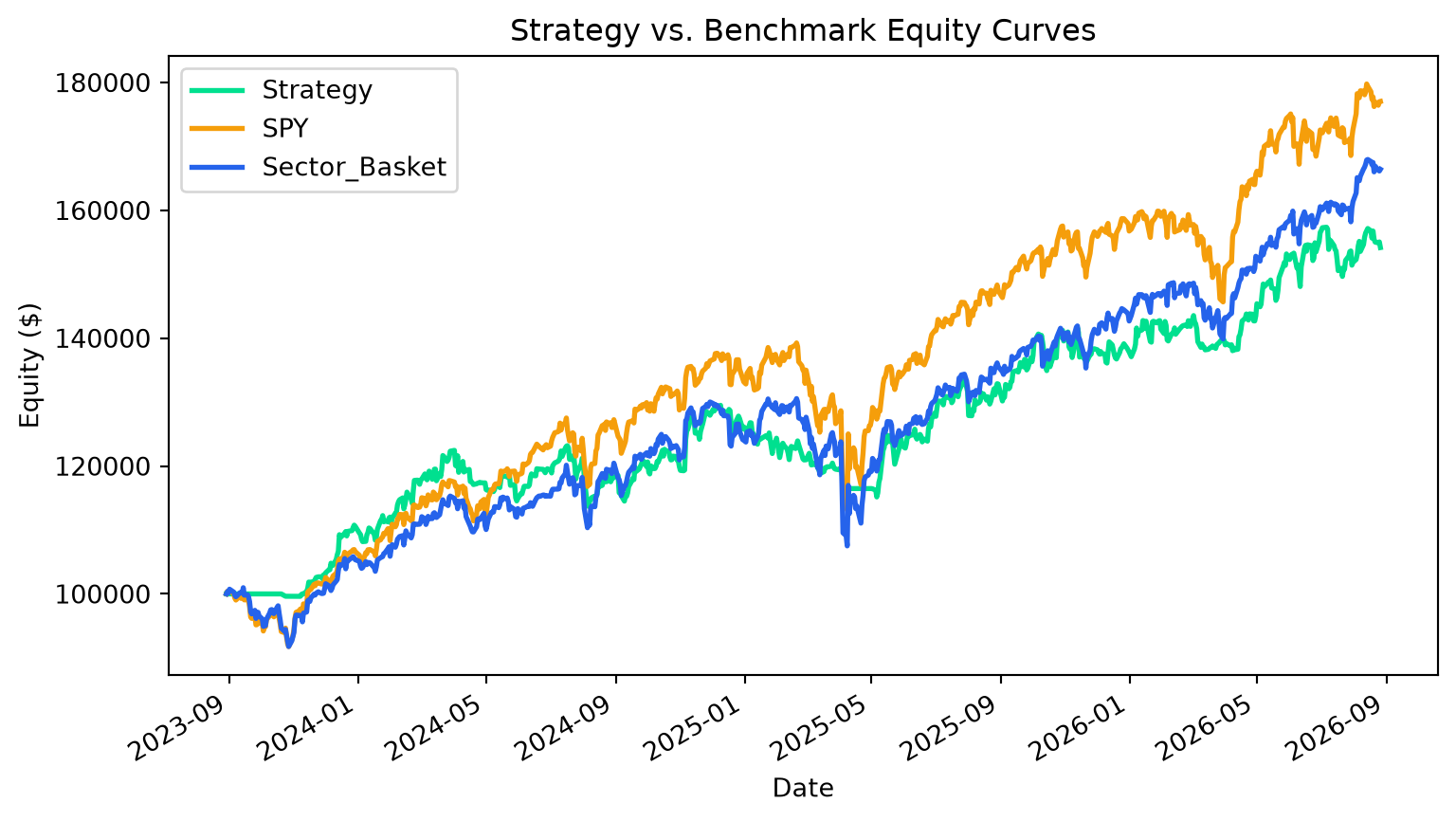
| Series | Final Equity | Total Return |
|---|---|---|
| Strategy | $154,175 | 54.17% |
| SPY | $177,038 | 77.04% |
| Sector_Basket | $166,418 | 66.42% |
The active strategy is compared against two passive benchmarks: buying and holding SPY, and an equal-weight buy-and-hold basket of all six sector ETFs.
sim_cash = portfolio.cash()
total_sim_value = portfolio.value()
exposure_pct = 100 * (1 - sim_cash / total_sim_value)

fig, ax = plt.subplots(figsize=(9, 5))
exposure_pct.plot(ax=ax, color="#00E08F", linewidth=1.5)
ax.axhline(0, linestyle="--", color="gray")
ax.set_title("Portfolio Exposure Over Time")
ax.set_ylabel("% of Equity Invested")
plt.show()
print(f"Average invested exposure: {exposure_pct.mean():.1f}%")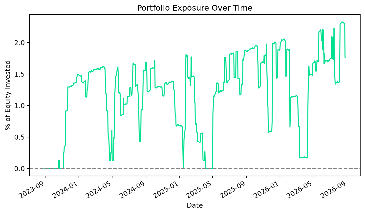
Average invested exposure: 1.2%Because every position is a fixed 300-share order rather than a percentage-of-equity allocation, exposure is not capped at 100%: once gains compound, several simultaneously-held winning positions can be worth more than the account’s starting equity.
bh_returns = (close.iloc[-1] / close.iloc[0] - 1) * 100| Symbol | Buy & Hold Return (%) |
|---|---|
| XLK | 114.98 |
| XLF | 77.12 |
| XLI | 73.98 |
| XLE | 55.46 |
| XLV | 35.25 |
| XLY | 41.71 |
# BIL = 1-3 month T-Bill ETF (near-zero duration); BND = intermediate-duration
# bonds; TLT = long-duration Treasuries.
cash_real = sim_cash - init_cash_sim + init_cash

def bond_overlay(bond_symbol):
    bond_close = vbt.YFData.download(bond_symbol, start=start_date, end=end_date).get('Close')
    bond_close = bond_close[bond_close.index.date >= start_calendar_date]
    bond_ret = bond_close.pct_change().reindex(cash_real.index).fillna(0)
    cash_flow = cash_real.diff()
    cash_flow.iloc[0] = 0
    cash_bond = cash_real.copy()
    for i in range(1, len(cash_bond)):
        cash_bond.iloc[i] = cash_bond.iloc[i - 1] * (1 + bond_ret.iloc[i]) + cash_flow.iloc[i]
    new_equity = cash_bond + (strategy_equity - cash_real)
    new_ret = new_equity.pct_change().dropna()
    total_return_ = (new_equity.iloc[-1] / init_cash - 1) * 100
    sharpe_ = new_ret.mean() / new_ret.std() * (252 ** 0.5)
    max_dd_ = -((new_equity / new_equity.cummax()) - 1).min() * 100
    return total_return_, sharpe_, max_dd_

overlay_rows = [{"Overlay": "Baseline", "Total Return %": total_ret, "Sharpe": sharpe, "Max DD %": maxdd}]
for sym in ["BIL", "BND", "TLT"]:
    tr, sh, dd = bond_overlay(sym)
    overlay_rows.append({"Overlay": sym, "Total Return %": tr, "Sharpe": sh, "Max DD %": dd})
overlay_df = pd.DataFrame(overlay_rows).round(2)| Overlay | Total Return % | Sharpe | Max DD % |
|---|---|---|---|
| Baseline | 54.17 | 1.28 | 11.07 |
| BIL | 54.99 | 1.30 | 10.33 |
| BND | 52.54 | 1.22 | 11.37 |
| TLT | 43.50 | 0.90 | 15.84 |
rolling_sharpe = strategy_ret.rolling(63).apply(lambda x: x.mean() / x.std() * np.sqrt(252), raw=True)

fig, ax = plt.subplots(figsize=(9, 5))
rolling_sharpe.plot(ax=ax, color="#00E08F")
ax.axhline(0, linestyle="--", color="gray")
ax.set_title("Rolling 3-Month Annualized Sharpe Ratio")
plt.show()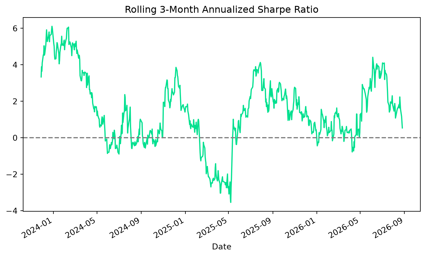
drawdown = (strategy_equity / strategy_equity.cummax() - 1) * 100
dd = drawdown.copy()
troughs, in_dd = [], False
for date, val in dd.items():
    if val < 0 and not in_dd:
        in_dd, start, trough_val, trough_date = True, date, val, date
    elif val < 0 and in_dd:
        if val < trough_val:
            trough_val, trough_date = val, date
    elif val >= 0 and in_dd:
        in_dd = False
        troughs.append({"From": start.date(), "Trough": trough_date.date(), "To": date.date(), "Depth %": trough_val})
if in_dd:
    troughs.append({"From": start.date(), "Trough": trough_date.date(), "To": None, "Depth %": trough_val})
top5 = pd.DataFrame(troughs).sort_values("Depth %").head(5).reset_index(drop=True)
top5["Depth %"] = top5["Depth %"].round(2)| From | Trough | To | Depth % |
|---|---|---|---|
| 2024-12-10 | 2025-05-06 | 2025-07-03 | -11.07 |
| 2024-07-18 | 2024-08-06 | 2024-11-06 | -7.70 |
| 2024-04-02 | 2024-05-30 | 2024-07-15 | -6.46 |
| 2026-07-07 | 2026-07-21 | None | -4.89 |
| 2025-07-29 | 2025-08-04 | 2025-09-12 | -4.19 |
fig, ax = plt.subplots(figsize=(9, 5))
ax.plot(close.index, close["XLK"], color="#1a1714", linewidth=1, label="XLK Close")
ax.plot(close.index, ema_fast["XLK"], color="#2563EB", linewidth=1, label="10-day EMA")
ax.plot(close.index, ema_slow["XLK"], color="#D9603E", linewidth=1, label="30-day EMA")
buy_dates = close.index[entries["XLK"].fillna(False)]
sell_dates = close.index[exits["XLK"].fillna(False)]
ax.scatter(buy_dates, close.loc[buy_dates, "XLK"], marker="^", color="#00E08F", s=60, zorder=5, label="Entry")
ax.scatter(sell_dates, close.loc[sell_dates, "XLK"], marker="v", color="#B3392F", s=60, zorder=5, label="Exit")
ax.set_title("XLK Price, 10/30 EMA & Signals")
ax.legend(loc="upper left", fontsize=8)
plt.show()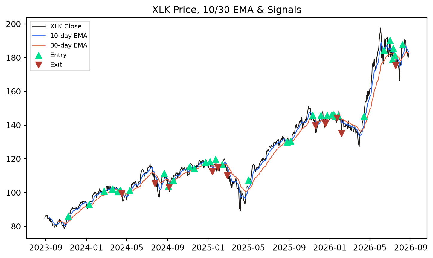
The grid search below optimizes over the entire backtest window with full hindsight. It is the right tool for mapping out the parameter surface, but its P&L numbers are not an honest performance estimate — the walk-forward section that follows is what actually tests whether this strategy design generalizes out-of-sample.
fast_grid = [5, 10, 15, 20]
slow_grid = [20, 30, 40, 50]
combos = [(f, s) for f in fast_grid for s in slow_grid if f < s]

def compute_signals(fast_n, slow_n, px):
    ema_f = px.apply(lambda col: ema(col, fast_n))
    ema_s = px.apply(lambda col: ema(col, slow_n))
    rsi_ = px.apply(lambda col: rsi(col, 14))
    state = ((ema_f > ema_s) & (rsi_ > 50)).astype(bool)
    prev = state.shift(1, fill_value=False).astype(bool)
    e = (state & ~prev).vbt.signals.fshift(1)
    x = ((ema_f < ema_s) & (ema_f.shift(1) >= ema_s.shift(1))).vbt.signals.fshift(1)
    return e, x

def run_window(fast_n, slow_n, win_start, win_end, cash_in, px, op):
    e_full, x_full = compute_signals(fast_n, slow_n, px)
    e, x = e_full.loc[win_start:win_end], x_full.loc[win_start:win_end]
    o = op.loc[win_start:win_end]
    return vbt.Portfolio.from_signals(o, entries=e, exits=x, price=o, init_cash=cash_in,
                                       cash_sharing=True, group_by=True, size=300,
size_type='amount', fees=0.0, slippage=0.0005, freq='1D')opt_rows = []
for fast_n, slow_n in combos:
pf = run_window(fast_n, slow_n, start_date, end_date, init_cash_sim, close, open_price)
opt_rows.append({"fast_n": fast_n, "slow_n": slow_n, "net_pl": pf.final_value() - init_cash_sim})
opt_df = pd.DataFrame(opt_rows).sort_values("net_pl", ascending=False).reset_index(drop=True)
opt_df["net_pl"] = opt_df["net_pl"].round(0)| fast_n | slow_n | net_pl |
|---|---|---|
| 10 | 40 | 59,602 |
| 5 | 50 | 58,779 |
| 10 | 20 | 58,273 |
| 15 | 30 | 54,916 |
| 15 | 20 | 54,580 |
| 5 | 40 | 54,566 |
| 10 | 30 | 54,175 |
| 5 | 30 | 52,503 |
| 10 | 50 | 50,082 |
| 20 | 30 | 49,320 |
| 15 | 40 | 49,272 |
| 15 | 50 | 49,088 |
| 20 | 40 | 48,218 |
| 5 | 20 | 44,670 |
| 20 | 50 | 43,344 |
Methodology. Every training score below is computed with Portfolio.from_signals restricted to exactly the training window’s dates — a position cannot be valued using a price from outside that window, because no later price is ever passed into that call. Each out-of-sample test window starts flat, carrying forward only the cash balance from the previous window’s end; this is a different (but equally look-ahead-free) convention from the R notebook’s continuous position carry, so the two walk-forward figures are not expected to match exactly.
wf_end_date = pd.Timestamp.today().strftime("%Y-%m-%d")
wf_data = vbt.YFData.download(symbols, start=start_date, end=wf_end_date)
wf_close = wf_data.get('Close')
wf_open = wf_data.get('Open')
wf_close = wf_close[wf_close.index.date >= start_calendar_date]
wf_open = wf_open[wf_open.index.date >= start_calendar_date]

month_end_mask = wf_close.index.to_series().groupby(
    [wf_close.index.year, wf_close.index.month]).transform('idxmax') == wf_close.index.to_series()
me_dates = wf_close.index[month_end_mask.values]

k_train, k_test = 18, 6
windows = []
w = 0
while (k_train + w * k_test) < len(me_dates):
    tr_end_i = k_train - 1 + w * k_test
    te_end_i = k_train - 1 + (w + 1) * k_test
    tr_start = wf_close.index[0] if w == 0 else me_dates[w * k_test - 1] + pd.Timedelta(days=1)
    tr_end = me_dates[tr_end_i]
    te_start = tr_end + pd.Timedelta(days=1)
    te_end = me_dates[te_end_i] if te_end_i < len(me_dates) else wf_close.index[-1]
    if te_start > wf_close.index[-1]:
        break
    windows.append((tr_start, tr_end, te_start, te_end))
    w += 1

windows_df = pd.DataFrame(windows, columns=["training_start", "training_end", "testing_start", "testing_end"])| training_start | training_end | testing_start | testing_end |
|---|---|---|---|
| 2023-08-29 04:00:00+00:00 | 2025-01-31 05:00:00+00:00 | 2025-02-01 05:00:00+00:00 | 2025-07-31 04:00:00+00:00 |
| 2024-02-01 05:00:00+00:00 | 2025-07-31 04:00:00+00:00 | 2025-08-01 04:00:00+00:00 | 2026-01-30 05:00:00+00:00 |
| 2024-08-01 04:00:00+00:00 | 2026-01-30 05:00:00+00:00 | 2026-01-31 05:00:00+00:00 | 2026-07-31 04:00:00+00:00 |
| 2025-02-01 05:00:00+00:00 | 2026-07-31 04:00:00+00:00 | 2026-08-01 04:00:00+00:00 | 2026-09-29 04:00:00+00:00 |
chosen_rows = []
oos_equity_parts = []
running_cash = init_cash
for (tr_start, tr_end, te_start, te_end) in windows:
    best_combo, best_obj = None, -np.inf
    for fast_n, slow_n in combos:
        pf_train = run_window(fast_n, slow_n, tr_start, tr_end, init_cash_sim, wf_close, wf_open)
        obj = pf_train.final_value() - init_cash_sim
        if obj > best_obj:
            best_obj, best_combo = obj, (fast_n, slow_n)
    chosen_rows.append({"training_start": tr_start.date(), "training_end": tr_end.date(),
                         "fast_n": best_combo[0], "slow_n": best_combo[1], "train_pl": round(best_obj, 0)})

    pf_test = run_window(best_combo[0], best_combo[1], te_start, te_end, init_cash_sim, wf_close, wf_open)
    window_equity = pf_test.value() - init_cash_sim + running_cash
    oos_equity_parts.append(window_equity)
    running_cash = float(window_equity.iloc[-1])

chosen_df = pd.DataFrame(chosen_rows)| training_start | training_end | fast_n | slow_n | train_pl |
|---|---|---|---|---|
| 2023-08-29 | 2025-01-31 | 10 | 20 | 28,569 |
| 2024-02-01 | 2025-07-31 | 10 | 20 | 20,370 |
| 2024-08-01 | 2026-01-30 | 5 | 50 | 24,419 |
| 2025-02-01 | 2026-07-31 | 5 | 50 | 35,277 |
oos_equity = pd.concat(oos_equity_parts)
oos_equity = oos_equity[~oos_equity.index.duplicated(keep="last")]
live_start, oos_end = oos_equity.index[0], oos_equity.index[-1]

wf_total_ret = (oos_equity.iloc[-1] / init_cash - 1) * 100
oos_ret = oos_equity.pct_change().dropna()
wf_sharpe = oos_ret.mean() / oos_ret.std() * np.sqrt(252)
wf_maxdd = -((oos_equity / oos_equity.cummax()) - 1).min() * 100print(f"Walk-forward out-of-sample: ${oos_equity.iloc[-1]:,.0f} "
f"({wf_total_ret:.1f}%), Sharpe {wf_sharpe:.2f}, Max DD {wf_maxdd:.1f}% "
f"over {live_start.date()} to {oos_end.date()}")Walk-forward out-of-sample: $133,821 (33.8%), Sharpe 1.40, Max DD 8.5% over 2025-02-03 to 2026-09-29Everything below is measured over the same dates — from the first out-of-sample day to the last — with every series rebased to start at zero.
def perf_stats(series):
    s = series.dropna()
    r = s.pct_change().dropna()
    return pd.Series({
        "Total_Return_Pct": (s.iloc[-1] / s.iloc[0] - 1) * 100,
        "Ann_Sharpe": r.mean() / r.std() * np.sqrt(252),
        "Max_Drawdown_Pct": -((s / s.cummax()) - 1).min() * 100
    })

fixed_pf = run_window(10, 30, live_start, oos_end, init_cash_sim, wf_close, wf_open)
fixed_equity = fixed_pf.value() - init_cash_sim + init_cash

hind_rows = []
for fast_n, slow_n in combos:
    pf = run_window(fast_n, slow_n, live_start, oos_end, init_cash_sim, wf_close, wf_open)
    hind_rows.append((fast_n, slow_n, pf.final_value()))
hb = max(hind_rows, key=lambda r: r[2])
hind_pf = run_window(hb[0], hb[1], live_start, oos_end, init_cash_sim, wf_close, wf_open)
hind_equity = hind_pf.value() - init_cash_sim + init_cash

spy_wf = vbt.YFData.download("SPY", start=start_date, end=wf_end_date).get('Close')
spy_wf = spy_wf[spy_wf.index.date >= start_calendar_date].loc[live_start:oos_end]
basket_wf = ((wf_close.loc[live_start:oos_end]) / wf_close.loc[live_start]).mean(axis=1) * init_cash

wf_comparison = pd.DataFrame({
    "Walk-forward (out-of-sample)": perf_stats(oos_equity),
    "Fixed EMA 10/30 (baseline rule)": perf_stats(fixed_equity),
    f"Hindsight-best fixed {hb[0]}/{hb[1]} (unattainable live)": perf_stats(hind_equity),
    "SPY buy & hold": perf_stats(spy_wf),
    "Equal-weight sector basket": perf_stats(basket_wf),
}).T.round(2)| Total_Return_Pct | Ann_Sharpe | Max_Drawdown_Pct | |
|---|---|---|---|
| Walk-forward (out-of-sample) | 33.82 | 1.40 | 8.53 |
| Fixed EMA 10/30 (baseline rule) | 34.58 | 1.34 | 8.43 |
| Hindsight-best fixed 10/40 (unattainable live) | 40.04 | 1.51 | 7.76 |
| SPY buy & hold | 30.35 | 1.02 | 18.76 |
| Equal-weight sector basket | 28.32 | 1.05 | 17.40 |
def rebase(s):
    return s / s.iloc[0] * 100 - 100

fig, ax = plt.subplots(figsize=(9, 5.5))
rebase(spy_wf).plot(ax=ax, color="#F59E0B", linewidth=2, label="SPY Buy & Hold")
rebase(basket_wf).plot(ax=ax, color="#2563EB", linewidth=2, label="Sector Basket Buy & Hold")
rebase(fixed_equity).plot(ax=ax, color="gray", linewidth=2, linestyle="--", label="Fixed EMA 10/30 (baseline rule)")
rebase(oos_equity).plot(ax=ax, color="#00E08F", linewidth=3, label="Walk-forward (params re-chosen each window)")
for _, row in chosen_df.iterrows():
    ax.axvline(pd.Timestamp(row["training_end"]) + pd.Timedelta(days=1), color="gray", linestyle=":", alpha=0.5)
ax.set_title("Walk-Forward Out-of-Sample Return vs. Benchmarks (same start date)")
ax.set_ylabel("Cumulative Return (%)")
ax.legend(loc="upper left", fontsize=8)
plt.figtext(0.5, -0.02, "Dotted vertical lines = re-optimization dates (start of each test window)",
            ha="center", fontsize=8, color="gray")
plt.show()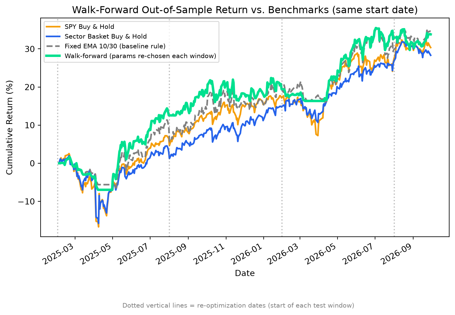
Over datetime.date(2025, 2, 3) to datetime.date(2026, 9, 29), the walk-forward strategy — re-choosing its EMA parameters every 6 months using only the preceding 18 months of data, with no look-ahead — returned 33.8%, versus 30.4% for SPY buy-and-hold and 34.6% for the simple fixed 10/30 rule held unchanged over the same dates.
Only relevant if you’re trying to reproduce this notebook and something doesn’t run the same way.
Python 3.11.16 | packaged by Anaconda, Inc. | (main, Aug 27 2026, 14:36:16) [MSC v.1942 64 bit (AMD64)]
Platform: Windows-10-10.0.26200-SP0
vectorbt: 1.1.1
pandas: 3.0.6
numpy: 2.4.6
matplotlib: 3.11.2
yfinance: 1.7.0
This notebook and its underlying strategy are for research and educational purposes only and do not constitute investment advice. Backtested and historical performance is not a guarantee or reliable indicator of future results. See quantstr.at for the full published article and additional strategy research.