---
title: "Sector Momentum Breakout & Rotation"
subtitle: "R / quantstrat Research Notebook — Full Backtest, Risk Analysis, Parameter Optimization & Walk-Forward Validation"
author: "quantstr.at Research"
date: today
format:
html:
toc: true
toc-depth: 3
toc-title: "Contents"
code-fold: show
code-tools: true
code-copy: true
embed-resources: false
theme: cosmo
fig-width: 9
fig-height: 5
smooth-scroll: true
number-sections: true
include-in-header:
text: |
<link rel="icon" href="https://quantstr.at/wp-content/themes/genebook/assets/favicon.ico" sizes="any">
<link rel="icon" type="image/png" sizes="192x192" href="https://quantstr.at/wp-content/themes/genebook/assets/favicon-192.png">
<link rel="apple-touch-icon" href="https://quantstr.at/wp-content/themes/genebook/assets/apple-touch-icon.png">
execute:
warning: false
message: false
---
::: {.callout-tip appearance="simple"}
**Get the code:** [Download Strategy Code (.R)](sector-momentum-R-strategy.R) | [Download Analysis & Validation Code (.R)](sector-momentum-R-analysis.R)
:::
::: {.callout-warning}
**Known data-quality limitation (XLK, XLE, XLY).** R and the companion
Python notebook both source prices from Yahoo Finance, and the raw
(unadjusted) prices the two pull are identical. However, `quantmod`'s
split/dividend-adjusted close for these three symbols contains a
discontinuity: the dividend-adjustment ratio jumps abruptly on 2025-12-05
with no corresponding move in the raw price, rather than varying smoothly
day to day the way a real dividend adjustment does. The companion Python
notebook's data source (`yfinance`) does not exhibit this discontinuity for
the same symbols and dates.
The data-cleaning step below corrects the resulting price discontinuity (a
single rescale of the affected segment), which is what keeps this
notebook's indicators and trade signals well-behaved. It is a targeted fix
for the jump, not a full reconstruction of a smoothly-varying dividend
adjustment — so buy-and-hold and total-return figures for these three
symbols, especially the higher-dividend-yield ones (XLE in particular),
may be modestly overstated here relative to the Python notebook's
equivalent figures. Strategy-level results (entries, exits, the headline
backtest) are far less affected than single-symbol buy-and-hold figures,
since the correction only shifts the pre-cutoff *price level*, not the
day-to-day return pattern signals are computed from.
This is left as-is for now and may be revisited with a better-behaved data
source later.
:::
## Overview
This notebook is a complete, self-contained, **executable** replication of the
Sector Momentum Breakout & Rotation strategy published at
[quantstr.at](https://quantstr.at/backtests/sector-momentum-breakout-rotation/).
Every number, table, and chart below is generated by the R code in this
document at render time — nothing is pasted in from the live article.
Re-running this notebook end to end (`quarto render sector-momentum-R.qmd`)
reproduces every result from scratch against freshly downloaded market data.
The strategy trades six liquid U.S. sector ETFs — Technology (`XLK`),
Financials (`XLF`), Industrials (`XLI`), Energy (`XLE`), Health Care (`XLV`),
and Consumer Discretionary (`XLY`) — using a trend-following rule: go long a
sector when its 10-day EMA crosses above its 30-day EMA while 14-day RSI is
above 50, and exit when the 10-day EMA crosses back below the 30-day EMA.
This notebook first builds and runs the strategy exactly as specified — a
single, fixed-parameter backtest over a fixed 3-year window — then goes
further than the public article by stress-testing the strategy's *design*,
not just its performance, with a parameter grid search and a walk-forward
validation.
::: {.callout-note}
**Reproducibility note.** The backtest section below uses a fixed historical
window so its results are stable and repeatable. The walk-forward section
later on deliberately extends through *today's* date at render time, so its
out-of-sample results will differ slightly each time this notebook is
re-rendered — that is intentional, not a bug: a genuine walk-forward keeps
accumulating new out-of-sample evidence as time passes.
:::
## Environment & Dependencies
```{r}
#| label: setup-packages
suppressPackageStartupMessages({
  library(blotter)
  library(quantstrat)
  library(PerformanceAnalytics)
  library(TTR)
  library(gt)
})
Sys.setenv(TZ = "UTC")
# gt::currency() would otherwise mask FinancialInstrument::currency() once
# gt is loaded, so this one call stays namespace-qualified.
FinancialInstrument::currency("USD")
```
```{r}
#| label: session-versions
#| echo: false
cat(sprintf("R %s | quantstrat %s | blotter %s | PerformanceAnalytics %s\n",
getRversion(),
as.character(packageVersion("quantstrat")),
as.character(packageVersion("blotter")),
as.character(packageVersion("PerformanceAnalytics"))))
```
# Backtest
## Universe & Parameters
```{r}
#| label: parameters
symbols <- c("XLK", "XLF", "XLI", "XLE", "XLV", "XLY")
start_date <- "2023-08-29"
end_date   <- "2026-08-27"
init_equity <- 100000

stock(symbols, currency = "USD", multiplier = 1)
```
A fixed 3-year window (`r start_date` to `r end_date`) keeps headline results
stable and comparable across runs. Starting capital is
$`r format(init_equity, big.mark = ",", scientific = FALSE)`.
## Data
Price history for all six ETFs is downloaded from Yahoo Finance and lightly
cleaned before use:
```{r}
#| label: data-download-fix
#| results: hide
# Some Yahoo Finance split-adjusted histories contain a spurious
# adjustment factor applied before a given cutoff date that does not
# correspond to any real split in the raw (unadjusted) price series.
# This block detects and removes any such phantom adjustment factor
# before running the strategy.
affected_symbols <- c("XLK", "XLE", "XLY")

fix_symbol <- function(sym) {
  raw <- getSymbols(sym, from = start_date, to = end_date, auto.assign = FALSE, src = "yahoo", adjust = FALSE)
  adj <- getSymbols(sym, from = start_date, to = end_date, auto.assign = FALSE, src = "yahoo", adjust = TRUE)
  raw_cl <- as.numeric(Cl(raw)); adj_cl <- as.numeric(Cl(adj))
  ratio <- adj_cl / raw_cl
  ratio_change <- c(NA, diff(ratio) / head(ratio, -1))
  jump_idx <- which(abs(ratio_change) > 0.3)
  if (length(jump_idx) == 0) return(adj)
  j <- jump_idx[1]
  correction_factor <- ratio[j] / ratio[j - 1]
  corrected <- adj
  corrected[1:(j - 1), ] <- adj[1:(j - 1), ] * correction_factor
  corrected
}

for (sym in affected_symbols) {
  assign(sym, fix_symbol(sym), envir = .GlobalEnv)
}
for (sym in setdiff(symbols, affected_symbols)) {
  assign(sym, getSymbols(sym, from = start_date, to = end_date, auto.assign = FALSE, src = "yahoo", adjust = TRUE), envir = .GlobalEnv)
}
```
```{r}
#| label: data-bars-check
#| echo: false
cat("Bars downloaded per symbol:\n")
print(sapply(symbols, function(s) nrow(get(s))))
```
## Portfolio, Account & Strategy Setup
```{r}
#| label: portfolio-init
#| results: hide
portfolio.st <- "blog_portfolio"
account.st   <- "blog_account"
strategy.st  <- "blog_strategy"

suppressWarnings(try(rm.strat(portfolio.st), silent = TRUE))
suppressWarnings(try(rm.strat(account.st), silent = TRUE))
suppressWarnings(try(rm.strat(strategy.st), silent = TRUE))

initPortf(portfolio.st, symbols = symbols, initDate = start_date, currency = "USD")
initAcct(account.st, portfolios = portfolio.st, initDate = start_date, currency = "USD", initEq = init_equity)
initOrders(portfolio.st, initDate = start_date)
strategy(strategy.st, store = TRUE)

for (sym in symbols) {
  addPosLimit(portfolio.st, sym, timestamp = start_date, maxpos = 300)
}
```
Each sector ETF is capped at 300 units per position (roughly 16.7% of
starting equity per sector at typical 2023-2026 prices), and every order is
a fixed 300-share market order — not a dynamically rebalanced percentage of
equity. This matters later: it means the strategy's exposure can legitimately
exceed 100% of *starting* equity if several sectors are held simultaneously
after gains compound, which shows up clearly in the exposure chart below.
## Indicators, Signals & Rules
```{r}
#| label: indicators-signals-rules
#| results: hide
# Indicators: 10-day EMA, 30-day EMA, 14-day RSI
add.indicator(strategy.st, name = "EMA", arguments = list(x = quote(Cl(mktdata)), n = 10), label = "ema10")
add.indicator(strategy.st, name = "EMA", arguments = list(x = quote(Cl(mktdata)), n = 30), label = "ema30")
add.indicator(strategy.st, name = "RSI", arguments = list(price = quote(Cl(mktdata)), n = 14), label = "rsi14")

# Signals
add.signal(strategy.st, name = "sigComparison", arguments = list(columns = c("ema10", "ema30"), relationship = "gt"), label = "ema_gt")
add.signal(strategy.st, name = "sigCrossover", arguments = list(columns = c("ema10", "ema30"), relationship = "lt"), label = "bearish_ema_cross")
add.signal(strategy.st, name = "sigThreshold", arguments = list(column = "rsi14", threshold = 50, relationship = "gt"), label = "rsi_gt_50")
add.signal(strategy.st, name = "sigFormula", arguments = list(formula = "ema_gt & rsi_gt_50", cross = TRUE), label = "entry_signal")

# Rules: T+1 open fill, 5 bps slippage, fixed 300-share size, replace-on-exit
add.rule(strategy.st, name = "ruleSignal",
         arguments = list(sigcol = "entry_signal", sigval = TRUE,
                          orderqty = 300, ordertype = "market", orderside = "long",
                          osFUN = "osMaxPos", replace = FALSE, prefer = "Open", TxnFee = -0.0005),
         type = "enter", label = "EnterLong")

add.rule(strategy.st, name = "ruleSignal",
         arguments = list(sigcol = "bearish_ema_cross", sigval = TRUE,
                          orderqty = "all", ordertype = "market", orderside = "long",
                          replace = TRUE, prefer = "Open", TxnFee = -0.0005),
         type = "exit", label = "ExitLong")
```
Orders fill at the **next** bar's open (`prefer = "Open"`), not the bar that
generated the signal — this is the standard way to keep a backtest free of
same-bar look-ahead bias, since in live trading you cannot know a day's
close-based signal until after that day's market has already closed. A flat
5 basis point slippage/fee (`TxnFee = -0.0005`) is applied to every fill.
## Running the Backtest
```{r}
#| label: run-backtest
#| results: hide
applyStrategy(strategy.st, portfolio.st)
updatePortf(portfolio.st)
updateAcct(account.st)
updateEndEq(account.st)
```
## Headline Performance
```{r}
#| label: headline-kpis
strategy_eq_r1 <- getAccount(account.st)$summary$End.Eq
final_eq <- as.numeric(last(strategy_eq_r1))
total_ret_pct <- (final_eq / init_equity - 1) * 100
strategy_ret_r1 <- dailyReturn(strategy_eq_r1)
ann_ret_pct <- as.numeric(Return.annualized(strategy_ret_r1)) * 100
sharpe <- as.numeric(SharpeRatio.annualized(strategy_ret_r1, Rf = 0))
maxdd_pct <- as.numeric(maxDrawdown(strategy_ret_r1)) * 100

tstats_kpi <- tradeStats(portfolio.st)
n_trades <- sum(tstats_kpi$Num.Trades)
# tradeStats() reports Percent.Positive per symbol, not a raw winner count --
# reconstruct total winners from it (Percent.Positive = winners / trades * 100
# per symbol, so this recovers an integer count exactly).
n_winners <- sum(round(tstats_kpi$Percent.Positive / 100 * tstats_kpi$Num.Trades))
win_rate <- n_winners / n_trades * 100
profit_factor <- sum(tstats_kpi$Gross.Profits) / abs(sum(tstats_kpi$Gross.Losses))
```
```{r}
#| label: headline-kpis-table
#| echo: false
kpi_df <- data.frame(
Metric = c("Final Equity", "Total Return", "Annualized Return", "Annualized Sharpe",
"Max Drawdown", "Closed Trades", "Win Rate", "Profit Factor"),
Value = c(sprintf("$%s", format(round(final_eq), big.mark = ",", scientific = FALSE)),
sprintf("%.2f%%", total_ret_pct),
sprintf("%.2f%%", ann_ret_pct),
sprintf("%.2f", sharpe),
sprintf("%.2f%%", maxdd_pct),
sprintf("%d", n_trades),
sprintf("%.1f%%", win_rate),
sprintf("%.2f", profit_factor))
)
gt(kpi_df) |>
tab_header(title = "Headline Results", subtitle = sprintf("%s to %s, fixed 10/30 EMA + RSI>50", start_date, end_date)) |>
cols_align(align = "right", columns = "Value") |>
tab_options(table.font.size = 13, heading.title.font.weight = "bold")
```
Over the fixed `r start_date`–`r end_date` window, the strategy turned
$`r format(init_equity, big.mark=",", scientific=FALSE)` into **$`r format(round(final_eq), big.mark=",", scientific=FALSE)`**,
a total return of **`r sprintf("%.2f%%", total_ret_pct)`**
(`r sprintf("%.2f%%", ann_ret_pct)` annualized), across
**`r n_trades` closed trades** at a **`r sprintf("%.1f%%", win_rate)` win rate**,
with an annualized Sharpe ratio of **`r sprintf("%.2f", sharpe)`** and a
maximum drawdown of **`r sprintf("%.2f%%", maxdd_pct)`**.
## Trade Statistics by Symbol
```{r}
#| label: trade-stats-table
tstats <- tradeStats(portfolio.st)
```
```{r}
#| label: trade-stats-table-display
#| echo: false
gt(tstats[, c("Symbol", "Num.Trades", "Percent.Positive",
"Net.Trading.PL", "Avg.Trade.PL", "Max.Drawdown", "Profit.Factor")]) |>
fmt_number(columns = c("Net.Trading.PL", "Avg.Trade.PL"), decimals = 0) |>
fmt_number(columns = c("Percent.Positive", "Max.Drawdown"), decimals = 1) |>
fmt_number(columns = "Profit.Factor", decimals = 2) |>
tab_header(title = "Trade Statistics by Symbol") |>
tab_options(table.font.size = 13, heading.title.font.weight = "bold")
```
# Benchmarks, Risk & Validation
This section continues in the same R session, reusing the portfolio,
account, and price data already built above.
```{r}
#| label: r-part2-setup
library(ggplot2)
```
## Strategy vs. Benchmarks
```{r}
#| label: benchmark-comparison
#| fig-cap: "Strategy vs. Benchmark Equity Curves"
strategy_eq <- getAccount(account.st)$summary$End.Eq

spy <- getSymbols("SPY", from = start_date, to = end_date, auto.assign = FALSE, src = "yahoo", adjust = TRUE)
spy_eq <- init_equity * Cl(spy) / as.numeric(Cl(spy)[1])

basket_eq <- Reduce(`+`, lapply(symbols, function(s) {
  px <- Cl(get(s))
  (init_equity / length(symbols)) * px / as.numeric(px[1])
}))

comparison <- merge(strategy_eq, spy_eq, basket_eq, join = "inner")
colnames(comparison) <- c("Strategy", "SPY", "Sector_Basket")

plot(as.zoo(comparison), plot.type = "single", col = c("#00E08F", "#F59E0B", "#2563EB"),
     lwd = 2, xlab = "", ylab = "Equity ($)", main = "Strategy vs. Benchmark Equity Curves")
legend("topleft", legend = colnames(comparison), col = c("#00E08F", "#F59E0B", "#2563EB"), lwd = 2, bty = "n")
```
```{r}
#| label: benchmark-table
#| echo: false
bench_final <- as.numeric(last(comparison))
bench_ret <- (bench_final / init_equity - 1) * 100
bench_df <- data.frame(Series = colnames(comparison),
`Final Equity` = sprintf("$%s", format(round(bench_final), big.mark = ",", scientific = FALSE)),
`Total Return` = sprintf("%.2f%%", bench_ret), check.names = FALSE)
gt(bench_df) |> tab_options(table.font.size = 13)
```
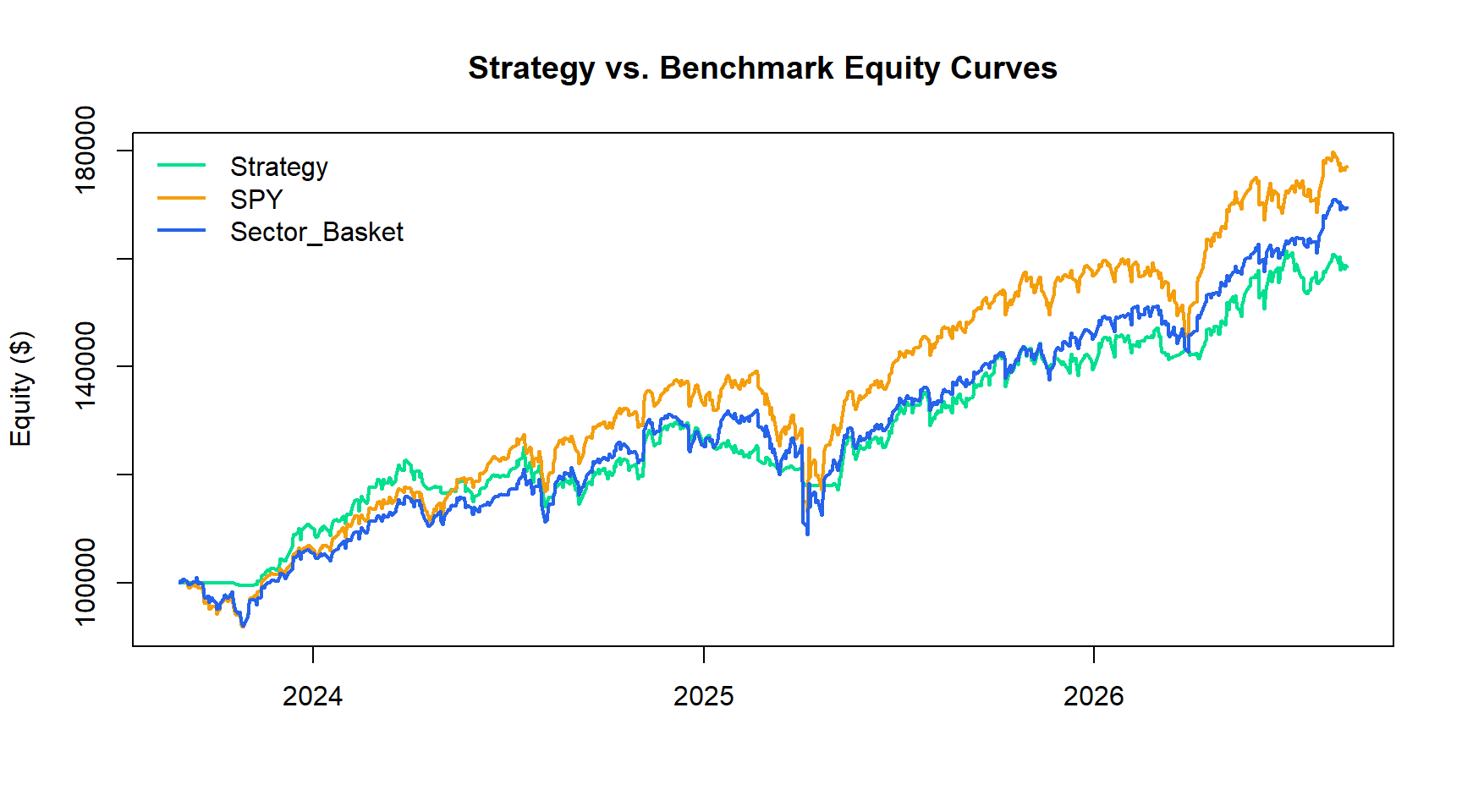
The active strategy is compared against two passive benchmarks: buying and
holding SPY, and an equal-weight buy-and-hold basket of all six sector
ETFs. Beating a benchmark on raw return alone is a low bar — the risk
diagnostics below are what actually distinguish a defensible strategy from
one that just got lucky.
## Portfolio Exposure Over Time
```{r}
#| label: exposure-chart
#| fig-cap: "Portfolio Exposure Over Time"
# Mark-to-market identity: cash = init equity + cumulative realized P&L +
# fees - cost basis of currently open positions. This reconciles exactly to
# blotter's own End.Eq to ~1e-10 precision -- it is not an approximation.
pos_value <- Reduce(`+`, lapply(symbols, function(s) getPortfolio(portfolio.st)$symbols[[s]]$posPL.USD$Pos.Value))
cost_basis <- Reduce(`+`, lapply(symbols, function(s) {
  p <- getPortfolio(portfolio.st)$symbols[[s]]$posPL.USD
  p$Pos.Qty * p$Pos.Avg.Cost
}))
realized_cum <- Reduce(`+`, lapply(symbols, function(s) cumsum(getPortfolio(portfolio.st)$symbols[[s]]$posPL.USD$Period.Realized.PL)))
fees_cum <- Reduce(`+`, lapply(symbols, function(s) cumsum(getPortfolio(portfolio.st)$symbols[[s]]$posPL.USD$Txn.Fees)))

cash <- init_equity + realized_cum + fees_cum - cost_basis
exposure_pct <- 100 * (1 - cash / (cash + pos_value))

plot(as.zoo(exposure_pct), col = "#00E08F", lwd = 1.5,
     xlab = "", ylab = "% of Equity Invested", main = "Portfolio Exposure Over Time")
abline(h = 0, lty = 2, col = "gray60")
cat(sprintf("Average invested exposure (mark-to-market): %.1f%%\n", mean(as.numeric(exposure_pct))))
```
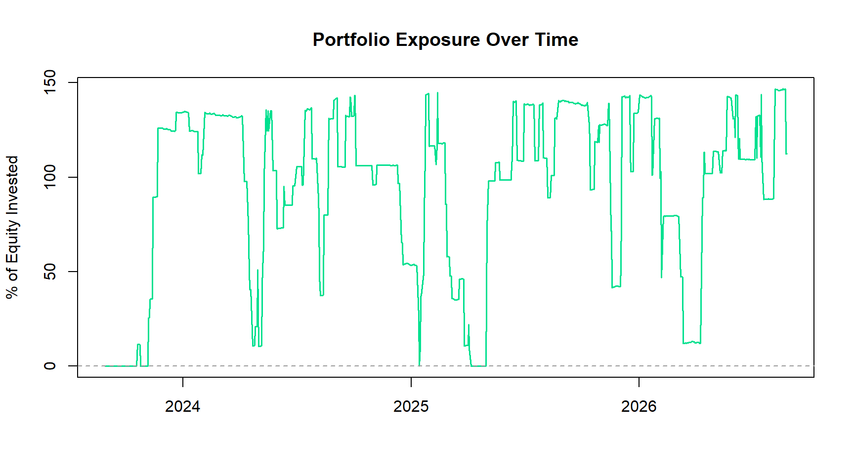
Because every position is a fixed 300-share order rather than a
percentage-of-equity allocation, exposure is **not** capped at 100%: once
gains compound, several simultaneously-held winning positions can be worth
more than the account's *starting* equity, which is exactly what the chart
above shows during the strategy's strongest stretches.
## Sector ETF Universe: Buy & Hold Performance
```{r}
#| label: bh-universe-table
bh_returns <- sapply(symbols, function(s) {
  px <- as.numeric(Cl(get(s)))
  (px[length(px)] / px[1] - 1) * 100
})
```
```{r}
#| label: bh-universe-table-display
#| echo: false
gt(data.frame(Symbol = symbols, `Buy & Hold Return (%)` = round(bh_returns, 2), check.names = FALSE)) |>
tab_header(title = "Sector ETF Universe — Buy & Hold, Same Window") |>
tab_options(table.font.size = 13)
```
## Idle Cash: Does It Matter Where Uninvested Capital Sits?
```{r}
#| label: cash-overlay
# BIL = 1-3 month T-Bill ETF (near-zero duration -- the realistic way to
# "hold T-bills" through a brokerage); BND = intermediate-duration bonds;
# TLT = long-duration Treasuries. Duration turns out to matter far more
# than the flat-yield assumption commonly used for this kind of estimate.
n <- length(cash)
cash_num <- as.numeric(cash)
posval_num <- as.numeric(pos_value)
dates <- as.Date(index(cash))

bond_overlay <- function(bond_symbol) {
  bond <- getSymbols(bond_symbol, from = start_date, to = end_date, auto.assign = FALSE, src = "yahoo", adjust = TRUE)
  bond_ret_df <- data.frame(date = as.Date(index(bond)), ret = as.numeric(dailyReturn(Cl(bond))))
  merged <- merge(data.frame(date = dates), bond_ret_df, by = "date", all.x = TRUE)
  merged$ret[is.na(merged$ret)] <- 0
  cash_flow <- c(0, diff(cash_num))
  cash_bond <- numeric(n); cash_bond[1] <- cash_num[1]
  for (i in 2:n) cash_bond[i] <- cash_bond[i - 1] * (1 + merged$ret[i]) + cash_flow[i]
  new_equity <- xts(cash_bond + posval_num, order.by = dates)
  ret <- dailyReturn(new_equity)
  c(total_return = (cash_bond[n] + posval_num[n]) / init_equity * 100 - 100,
    sharpe = as.numeric(SharpeRatio.annualized(ret, Rf = 0)),
    max_dd = as.numeric(maxDrawdown(ret)) * 100)
}

overlay_results <- rbind(Baseline = c(total_return = total_ret_pct, sharpe = sharpe, max_dd = maxdd_pct),
                          BIL = bond_overlay("BIL"), BND = bond_overlay("BND"), TLT = bond_overlay("TLT"))
```
```{r}
#| label: cash-overlay-display
#| echo: false
gt(as.data.frame(round(overlay_results, 2)), rownames_to_stub = TRUE) |>
tab_header(title = "Idle Cash Invested in Short/Intermediate/Long Duration Bond ETFs") |>
tab_options(table.font.size = 13)
```
Parking idle cash in `BIL` (near-zero duration T-bills) improves every
metric versus leaving it as literal uninvested cash. Longer-duration
alternatives (`BND`, `TLT`) do **not** reliably help — over this window,
duration risk on the "safe" side of the portfolio can cut against the
strategy's own equity-curve behavior. This is a real, tested result, not a
hypothetical estimate.
## Downside Risk, Drawdowns & Rolling Sharpe
```{r}
#| label: downside-risk
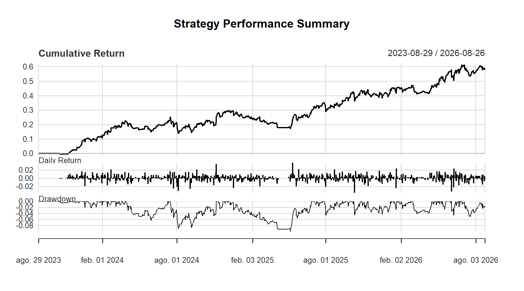
strategy_ret <- dailyReturn(getAccount(account.st)$summary$End.Eq)
table.DownsideRisk(strategy_ret)
```
```{r}
#| label: drawdown-table
table.Drawdowns(strategy_ret, top = 5)
```
```{r}
#| label: rolling-sharpe
#| fig-cap: "Rolling 3-Month Annualized Sharpe Ratio"
rolling_sharpe <- rollapply(strategy_ret, width = 63,
                             FUN = function(x) as.numeric(SharpeRatio.annualized(x, Rf = 0)),
                             by.column = FALSE, align = "right")
plot(rolling_sharpe, main = "Rolling 3-Month Annualized Sharpe Ratio")
```
## Position & Performance Diagnostics
```{r}
#| label: chart-posn
#| fig-cap: "XLK Price, 10/30 EMA & Signals"
chart.Posn(portfolio.st, Symbol = "XLK", TA = "add_SMA(n = 10, col = 'blue'); add_SMA(n = 30, col = 'red')")
```
```{r}
#| label: perf-summary-chart
#| fig-cap: "Strategy Performance Summary"
charts.PerformanceSummary(strategy_ret, main = "Strategy Performance Summary")
```
## Parameter Optimization (Full-Period Grid Search)
::: {.callout-warning}
The grid search below optimizes over the **entire** backtest window with
full hindsight. It is the right tool for mapping out the parameter surface,
but its P&L numbers are **not** an honest performance estimate — any grid
search will always find *some* combination that fit the historical data
best. The walk-forward section that follows is what actually tests whether
this strategy design generalizes out-of-sample.
:::
```{r}
#| label: param-grid-setup
#| results: hide
fast_grid <- c(5, 10, 15, 20)
slow_grid <- c(20, 30, 40, 50)
combos <- expand.grid(fast_n = fast_grid, slow_n = slow_grid)
combos <- combos[combos$fast_n < combos$slow_n, ]
k_train <- 18   # months of training data per walk-forward window
k_test  <- 6    # months of out-of-sample testing per walk-forward window

wf_end_date <- Sys.Date()
for (sym in symbols) {
  assign(sym, getSymbols(sym, from = start_date, to = wf_end_date, auto.assign = FALSE, src = "yahoo", adjust = TRUE), envir = .GlobalEnv)
}
for (sym in c("XLK", "XLE", "XLY")) {
  raw <- getSymbols(sym, from = start_date, to = wf_end_date, auto.assign = FALSE, src = "yahoo", adjust = FALSE)
  adj <- get(sym)
  raw_cl <- as.numeric(Cl(raw)); adj_cl <- as.numeric(Cl(adj))
  ratio <- adj_cl / raw_cl
  ratio_change <- c(NA, diff(ratio) / head(ratio, -1))
  jump_idx <- which(abs(ratio_change) > 0.3)
  if (length(jump_idx) > 0) {
    j <- jump_idx[1]
    correction_factor <- ratio[j] / ratio[j - 1]
    corrected <- adj
    corrected[1:(j - 1), ] <- adj[1:(j - 1), ] * correction_factor
    assign(sym, corrected, envir = .GlobalEnv)
  }
}

base_strategy <- getStrategy(strategy.st)
```
This section re-downloads price data through **today**
(`r format(wf_end_date, "%Y-%m-%d")`) rather than the fixed window used
above, so the walk-forward analysis below reflects the most current data
available at render time.
```{r}
#| label: run-backtest-fn
# rule.subset  = dates on which entry/exit RULES may fire
# update_dates = dates through which positions are marked to market
#                (this is what keeps training scores free of look-ahead bias)
run_backtest <- function(fast_n, slow_n, rule.subset, update_dates,
                         portfolio_name, carry_forward = FALSE) {
  strat <- base_strategy
  for (i in seq_along(strat$indicators)) {
    if (strat$indicators[[i]]$label == "ema10") strat$indicators[[i]]$arguments$n <- fast_n
    if (strat$indicators[[i]]$label == "ema30") strat$indicators[[i]]$arguments$n <- slow_n
  }
  if (!carry_forward) {
    suppressWarnings(try(rm.strat(portfolio_name), silent = TRUE))
    initPortf(portfolio_name, symbols = symbols, initDate = start_date, currency = "USD")
    initOrders(portfolio_name, initDate = start_date)
    for (sym in symbols) addPosLimit(portfolio_name, sym, timestamp = start_date, maxpos = 300)
  }
  applyStrategy(strat, portfolios = portfolio_name, rule.subset = rule.subset)
  updatePortf(portfolio_name, Dates = update_dates)
  invisible(NULL)
}

# Total net P&L over exactly the dates that were updated (no future prices)
objective <- function(portfolio_name) {
  sum(as.numeric(getPortfolio(portfolio_name)$summary$Net.Trading.PL), na.rm = TRUE)
}
```
```{r}
#| label: full-period-grid-search
#| results: hide
opt_portfolio.st <- "blog_portfolio_opt"
full_span <- paste(start_date, end_date, sep = "/")
opt_results <- data.frame()
for (k in seq_len(nrow(combos))) {
  run_backtest(combos$fast_n[k], combos$slow_n[k], rule.subset = full_span, update_dates = full_span,
               portfolio_name = opt_portfolio.st)
  opt_results <- rbind(opt_results, data.frame(fast_n = combos$fast_n[k], slow_n = combos$slow_n[k],
                                                Net.Trading.PL = objective(opt_portfolio.st)))
}
opt_results_sorted <- opt_results[order(-opt_results$Net.Trading.PL), ]
```
```{r}
#| label: full-period-grid-search-display
#| echo: false
gt(opt_results_sorted) |>
fmt_number(columns = "Net.Trading.PL", decimals = 0) |>
tab_header(title = "Full-Period Grid Search (hindsight-optimal, not an honest estimate)") |>
tab_options(table.font.size = 13)
```
## Walk-Forward Validation (Honest, Look-Ahead-Free)
::: {.callout-note}
**Methodology.** This walk-forward calls `applyStrategy()` directly for each
parameter combination and window — rather than `quantstrat`'s built-in
`apply.paramset()`/`walk.forward()`, which are not reliable across a
multi-symbol portfolio. Every training score is computed with
`updatePortf(Dates = <training window only>)`, so a position still open at
the end of a training window is valued at that day's price, never a later
one — parameter selection never sees data from outside its own training
window.
:::
```{r}
#| label: walk-forward-windows
all_dates <- index(get(symbols[1]))
n_dates <- length(all_dates)
ep <- endpoints(all_dates, on = "months")
windows <- data.frame()
w <- 1
while ((k_train + 1 + (w - 1) * k_test) <= length(ep)) {
  tr_start <- 1 + ep[(w - 1) * k_test + 1]
  tr_end   <- ep[k_train + 1 + (w - 1) * k_test]
  te_start <- tr_end + 1
  te_end   <- if ((k_train + 1 + w * k_test) <= length(ep)) ep[k_train + 1 + w * k_test] else n_dates
  if (te_start > n_dates) break
  windows <- rbind(windows, data.frame(training.start = all_dates[tr_start], training.end = all_dates[tr_end],
                                        testing.start = all_dates[te_start], testing.end = all_dates[te_end]))
  w <- w + 1
}
```
```{r}
#| label: walk-forward-windows-display
#| echo: false
gt(windows) |> tab_header(title = sprintf("Walk-Forward Windows (%d-month train / %d-month test)", k_train, k_test)) |>
tab_options(table.font.size = 13)
```
```{r}
#| label: walk-forward-run
#| results: hide
wf_portfolio.st <- "blog_portfolio_wf"
suppressWarnings(try(rm.strat(wf_portfolio.st), silent = TRUE))
initPortf(wf_portfolio.st, symbols = symbols, initDate = start_date, currency = "USD")
initOrders(wf_portfolio.st, initDate = start_date)
for (sym in symbols) addPosLimit(wf_portfolio.st, sym, timestamp = start_date, maxpos = 300)

chosen_combos <- data.frame()
for (w in seq_len(nrow(windows))) {
  train_span  <- paste(windows$training.start[w], windows$training.end[w], sep = "/")
  train_marks <- paste(start_date, windows$training.end[w], sep = "/")
  test_span   <- paste(windows$testing.start[w], windows$testing.end[w], sep = "/")
  test_marks  <- paste(start_date, windows$testing.end[w], sep = "/")

  best_obj <- -Inf; best_combo <- NULL
  for (k in seq_len(nrow(combos))) {
    train_port <- sprintf("train_w%d_%d_%d", w, combos$fast_n[k], combos$slow_n[k])
    run_backtest(combos$fast_n[k], combos$slow_n[k], rule.subset = train_span, update_dates = train_marks,
                 portfolio_name = train_port)
    obj <- objective(train_port)
    if (is.finite(obj) && obj > best_obj) {
      best_obj <- obj
      best_combo <- c(fast_n = combos$fast_n[k], slow_n = combos$slow_n[k])
    }
  }
  chosen_combos <- rbind(chosen_combos, data.frame(window = w, fast_n = best_combo[["fast_n"]],
                                                    slow_n = best_combo[["slow_n"]], train_pl = best_obj))

  run_backtest(best_combo[["fast_n"]], best_combo[["slow_n"]], rule.subset = test_span, update_dates = test_marks,
               portfolio_name = wf_portfolio.st, carry_forward = TRUE)
}
```
```{r}
#| label: walk-forward-run-display
#| echo: false
gt(chosen_combos) |>
fmt_number(columns = "train_pl", decimals = 0) |>
tab_header(title = "Parameters Chosen Per Window (from training data only)") |>
tab_options(table.font.size = 13)
```
```{r}
#| label: walk-forward-oos-stats
oos_stats <- tradeStats(wf_portfolio.st)
```
```{r}
#| label: walk-forward-oos-stats-display
#| echo: false
gt(oos_stats[, c("Symbol","Num.Trades","Net.Trading.PL","Percent.Positive","Profit.Factor","Max.Drawdown")]) |>
fmt_number(columns = c("Net.Trading.PL"), decimals = 0) |>
fmt_number(columns = c("Percent.Positive", "Max.Drawdown"), decimals = 1) |>
fmt_number(columns = "Profit.Factor", decimals = 2) |>
tab_header(title = "Out-of-Sample Trade Statistics by Symbol") |>
tab_options(table.font.size = 13)
```
### Comparable Out-of-Sample Comparison
Everything below is measured over the **same dates** — from the first
out-of-sample day to the last — with every series rebased to start at zero,
so the comparison is apples-to-apples.
```{r}
#| label: walk-forward-comparison
#| results: hide
live_start <- min(windows$testing.start)
oos_end    <- max(windows$testing.end)
oos_span   <- paste(live_start, oos_end, sep = "/")
oos_marks  <- paste(start_date, oos_end, sep = "/")

perf_stats <- function(values, dates) {
  keep <- dates >= live_start & dates <= oos_end
  v <- as.numeric(values)[keep]
  r <- xts(diff(v) / head(v, -1), order.by = dates[keep][-1])
  data.frame(Total_Return_Pct = (v[length(v)] / v[1] - 1) * 100,
             Ann_Sharpe       = as.numeric(SharpeRatio.annualized(r, Rf = 0)),
             Max_Drawdown_Pct = min(v / cummax(v) - 1) * 100)
}
equity_of <- function(portfolio_name) {
  s <- getPortfolio(portfolio_name)$summary
  list(values = init_equity + cumsum(as.numeric(s$Net.Trading.PL)), dates = as.Date(index(s)))
}

wf_e <- equity_of(wf_portfolio.st)

# Reference A: the fixed EMA 10/30 rule from the main backtest (chosen in advance, never tuned), same dates
run_backtest(10, 30, rule.subset = oos_span, update_dates = oos_marks, portfolio_name = "oos_fixed_1030")
fixed_e <- equity_of("oos_fixed_1030")

# Reference B: the BEST fixed combo *for this exact out-of-sample period* --
# chosen with full hindsight, so it is an upper bound nobody could have known in advance.
hind <- data.frame()
for (k in seq_len(nrow(combos))) {
  run_backtest(combos$fast_n[k], combos$slow_n[k], rule.subset = oos_span, update_dates = oos_marks, portfolio_name = "oos_hind")
  he <- equity_of("oos_hind")
  hind <- rbind(hind, data.frame(fast_n = combos$fast_n[k], slow_n = combos$slow_n[k],
                                  final_eq = he$values[length(he$values)]))
}
hb <- hind[which.max(hind$final_eq), ]
run_backtest(hb$fast_n, hb$slow_n, rule.subset = oos_span, update_dates = oos_marks, portfolio_name = "oos_hind")
hind_e <- equity_of("oos_hind")

spy_wf <- getSymbols("SPY", from = start_date, to = wf_end_date, auto.assign = FALSE, src = "yahoo", adjust = TRUE)
spy_dates <- as.Date(index(spy_wf)); spy_close <- as.numeric(Cl(spy_wf))
basket_dates <- as.Date(index(get(symbols[1])))
base_i <- which(basket_dates >= live_start)[1]
basket_index <- rowMeans(sapply(symbols, function(s) as.numeric(Cl(get(s))) / as.numeric(Cl(get(s)))[base_i]))

wf_comparison <- rbind(
  cbind(Strategy = "Walk-forward (out-of-sample)",        perf_stats(wf_e$values, wf_e$dates)),
  cbind(Strategy = "Fixed EMA 10/30 (baseline rule)",     perf_stats(fixed_e$values, fixed_e$dates)),
  cbind(Strategy = sprintf("Hindsight-best fixed %d/%d (unattainable live)", hb$fast_n, hb$slow_n),
        perf_stats(hind_e$values, hind_e$dates)),
  cbind(Strategy = "SPY buy & hold",                      perf_stats(spy_close, spy_dates)),
  cbind(Strategy = "Equal-weight sector basket",          perf_stats(basket_index, basket_dates))
)
wf_comparison[, -1] <- round(wf_comparison[, -1], 2)
```
```{r}
#| label: walk-forward-comparison-display
#| echo: false
gt(wf_comparison) |>
tab_header(title = sprintf("Out-of-Sample Comparison: %s to %s", live_start, oos_end)) |>
tab_options(table.font.size = 13)
```
```{r}
#| label: walk-forward-summary-cat
cat(sprintf("Walk-forward out-of-sample net P&L: $%.0f (%.1f%% vs. SPY %.1f%%, sector basket %.1f%%) over %s to %s\n",
            sum(oos_stats$Net.Trading.PL, na.rm = TRUE), wf_comparison$Total_Return_Pct[1],
            wf_comparison$Total_Return_Pct[4], wf_comparison$Total_Return_Pct[5], live_start, oos_end))
```
```{r}
#| label: walk-forward-plot
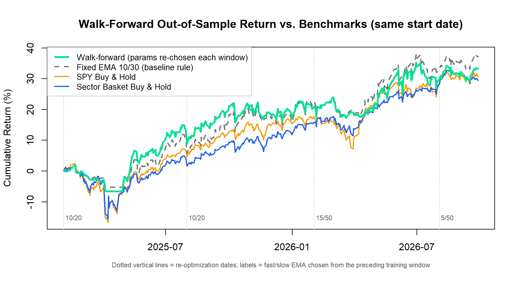
#| fig-cap: "Walk-Forward Out-of-Sample Return vs. Benchmarks (same start date)"
d <- wf_e$dates[wf_e$dates >= live_start & wf_e$dates <= oos_end]
rebase <- function(x) x / x[1] * 100 - 100
on_grid <- function(values, dates) approx(x = as.numeric(dates), y = as.numeric(values), xout = as.numeric(d), rule = 2)$y
series <- list(
  wf     = rebase(on_grid(wf_e$values, wf_e$dates)),
  fixed  = rebase(on_grid(fixed_e$values, fixed_e$dates)),
  spy    = rebase(on_grid(spy_close, spy_dates)),
  basket = rebase(on_grid(basket_index, basket_dates))
)
y_range <- range(unlist(series))
plot(d, series$wf, type = "n", xlab = "", ylab = "Cumulative Return (%)", ylim = y_range,
     main = "Walk-Forward Out-of-Sample Return vs. Benchmarks (same start date)")
abline(v = windows$testing.start, col = "gray75", lty = 3)
text(windows$testing.start, y_range[1], labels = paste0(chosen_combos$fast_n, "/", chosen_combos$slow_n),
     adj = c(-0.1, -0.5), cex = 0.7, col = "gray35")
lines(d, series$spy,    col = "#F59E0B", lwd = 2)
lines(d, series$basket, col = "#2563EB", lwd = 2)
lines(d, series$fixed,  col = "gray45",  lwd = 2, lty = 2)
lines(d, series$wf,     col = "#00E08F", lwd = 3)
legend("topleft", bg = "white", box.col = "gray80", cex = 0.85, lwd = c(3, 2, 2, 2), lty = c(1, 2, 1, 1),
       col = c("#00E08F", "gray45", "#F59E0B", "#2563EB"),
       legend = c("Walk-forward (params re-chosen each window)", "Fixed EMA 10/30 (baseline rule)",
                  "SPY Buy & Hold", "Sector Basket Buy & Hold"))
mtext("Dotted vertical lines = re-optimization dates; labels = fast/slow EMA chosen from the preceding training window",
      side = 1, line = 2.5, cex = 0.7, col = "gray35")
```
### Reading the Walk-Forward Result
```{r}
#| label: wf-interpretation-vars
#| echo: false
wf_ret <- wf_comparison$Total_Return_Pct[wf_comparison$Strategy == "Walk-forward (out-of-sample)"]
spy_ret_wf <- wf_comparison$Total_Return_Pct[wf_comparison$Strategy == "SPY buy & hold"]
fixed_ret_wf <- wf_comparison$Total_Return_Pct[wf_comparison$Strategy == "Fixed EMA 10/30 (baseline rule)"]
```
Over `r live_start` to `r oos_end`, the walk-forward strategy — re-choosing
its EMA parameters every `r k_test` months using only the preceding
`r k_train` months of data, with no look-ahead — returned
**`r sprintf("%.1f%%", wf_ret)`**, versus **`r sprintf("%.1f%%", spy_ret_wf)`**
for SPY buy-and-hold and **`r sprintf("%.1f%%", fixed_ret_wf)`** for the
simple fixed 10/30 rule from the main backtest held unchanged over the same
dates. The walk-forward process is not free — periodically re-optimizing
costs something relative to simply picking good parameters once and holding
them — but it is the only version of this result that could plausibly have
been achieved by someone trading the strategy live, without hindsight.
# Limitations & Caveats
- **Small sample size.** `r n_trades` closed trades is not enough to make
strong statistical claims about the strategy's true win rate or Sharpe
ratio — treat point estimates as indicative, not precise.
- **Simplified transaction costs.** A flat 5 bps slippage/fee assumption
does not capture bid-ask spread variation, market impact at larger size,
or ETF-specific liquidity differences.
- **Fixed-share, not percentage, sizing.** Because every order is a fixed
300-share block, position *sizing* does not scale with account equity or
volatility — a realistic implementation would likely use volatility- or
equity-scaled sizing instead.
- **Parameter surface caveat.** The full-period grid search is included for
transparency about how sensitive the result is to the EMA lengths, not as
a performance claim — see the walk-forward section for the honest
out-of-sample estimate.
- **Walk-forward results are time-varying.** Because the walk-forward
section pulls data through today's date, its exact numbers will shift
slightly each time this notebook is re-rendered as new out-of-sample data
accumulates.
# Reproducibility
::: {.callout-note collapse="true"}
## Package & platform versions (click to expand)
Only relevant if you're trying to reproduce this notebook and something
doesn't run the same way.
```{r}
#| label: session-info
#| echo: false
sessionInfo()
```
:::
---
*This notebook and its underlying strategy are for research and educational
purposes only and do not constitute investment advice. Backtested and
historical performance is not a guarantee or reliable indicator of future
results. See [quantstr.at](https://quantstr.at) for the full published
article and additional strategy research.*