Code
import numpy as np
import pandas as pd
import vectorbt as vbt

print(f"vectorbt {vbt.__version__} | pandas {pd.__version__} | numpy {np.__version__}")
vectorbt 1.1.1 | pandas 3.0.6 | numpy 2.4.6Python / VectorBT Research Notebook
Get the code: Download Strategy Code (.py) | Download Analysis Code (.py)
This notebook is a complete, executable Python replication of the strategy published at quantstr.at, built on VectorBT. Every number, table and chart below is produced by the Python code in this document at render time.
The strategy, as specified:
Trade QQQ, NVDA, AAPL, MSFT, AMD, and AMZN using a Keltner Channel Volatility Breakout strategy. The channel is a 20-period EMA centre line with upper and lower bands set 2.0 x the 10-period ATR away from it. Enter long when the close breaks above the upper band and the 14-period ADX is above 25 (confirming trend strength). Exit when the close falls below the 20-period EMA centre line.
Differences from the R report. The two engines are independent implementations. Small differences in results are expected: VectorBT sizes orders in fractional shares where the R report uses whole shares, and the two data libraries apply price adjustments separately.
import numpy as np
import pandas as pd
import vectorbt as vbt
print(f"vectorbt {vbt.__version__} | pandas {pd.__version__} | numpy {np.__version__}")vectorbt 1.1.1 | pandas 3.0.6 | numpy 2.4.6Same universe, window and sizing as the R report: one equal dollar slot per symbol, long-only, no leverage, no adding to an open position.
symbols = ["QQQ", "NVDA", "AAPL", "MSFT", "AMD", "AMZN"]
start_date = "2023-08-29"
end_date = "2026-08-27"
init_equity = 100_000

ema_n = 20       # Keltner centre line: EMA of the close
atr_n = 10       # Keltner band width: ATR period
atr_mult = 2.0   # Keltner band width: ATR multiplier
adx_n = 14       # trend-strength filter period
adx_min = 25     # entries require ADX above this level
slot_usd = init_equity / len(symbols)
cost_rate = 0.0005 # 5 bps of traded value on every fillDaily bars from Yahoo Finance via yfinance, with OHLC adjusted for splits and dividends.
data = vbt.YFData.download(symbols, start=start_date, end=end_date, missing_columns="nan")
close = data.get("Close")[symbols]
open_ = data.get("Open")[symbols]
high = data.get("High")[symbols]
low = data.get("Low")[symbols]

# Keep the same trading-day range as the R report (calendar-date filter).
in_range = close.index.date >= pd.Timestamp(start_date).date()
close, open_, high, low = close[in_range], open_[in_range], high[in_range], low[in_range]

worst = close.pct_change().abs().max()
assert (worst < 0.40).all(), f"suspect unadjusted split: {worst[worst >= 0.40].to_dict()}"
print("Bars downloaded per symbol:")
print(close.count())
Bars downloaded per symbol:
symbol
QQQ 751
NVDA 751
AAPL 751
MSFT 751
AMD 751
AMZN 751
dtype: int64EMA uses alpha = 2/(n+1) and Wilder smoothing uses alpha = 1/n; both are SMA-seeded, matching the R report’s TTR::EMA(), TTR::ATR() and TTR::ADX().
def sma_seeded(df: pd.DataFrame, n: int, alpha: float) -> pd.DataFrame:
    x = df.to_numpy(dtype=float)
    out = np.full(x.shape, np.nan)
    for j in range(x.shape[1]):
        col = x[:, j]
        valid = np.flatnonzero(~np.isnan(col))
        if len(valid) < n:
            continue
        s = valid[0] + n - 1
        out[s, j] = col[valid[0]:s + 1].mean()
        for i in range(s + 1, len(col)):
            out[i, j] = alpha * col[i] + (1 - alpha) * out[i - 1, j]
    return pd.DataFrame(out, index=df.index, columns=df.columns)

ema = lambda df, n: sma_seeded(df, n, 2.0 / (n + 1))
wilder = lambda df, n: sma_seeded(df, n, 1.0 / n)

prev_close = close.shift(1)
true_range = pd.DataFrame(
    np.maximum.reduce([(high - low).to_numpy(), (high - prev_close).abs().to_numpy(), (low - prev_close).abs().to_numpy()]),
    index=close.index, columns=close.columns)
true_range.iloc[0] = (high - low).iloc[0]

mid = ema(close, ema_n)
atr = wilder(true_range, atr_n)
upper = mid + atr_mult * atr
lower = mid - atr_mult * atr

up_move = high.diff()
down_move = -low.diff()
plus_dm = up_move.where((up_move > down_move) & (up_move > 0), 0.0)
minus_dm = down_move.where((down_move > up_move) & (down_move > 0), 0.0)
tr_adx = wilder(true_range, adx_n)
di_pos = 100 * wilder(plus_dm, adx_n) / tr_adx
di_neg = 100 * wilder(minus_dm, adx_n) / tr_adx
dx = 100 * (di_pos - di_neg).abs() / (di_pos + di_neg)
adx = wilder(dx.dropna(how="all"), adx_n).reindex(close.index)Entry fires on the first bar where the close is above the upper band AND ADX is above its threshold. Exit fires when the close crosses below the EMA centre line. A signal evaluated on day T is executed at day T+1’s open.
entry_state = ((close > upper) & (adx > adx_min)).fillna(False).astype(bool)
raw_entries = entry_state & ~entry_state.shift(1, fill_value=False)
raw_exits = ((close < mid) & (close.shift(1) >= mid.shift(1))).fillna(False).astype(bool)

entries = raw_entries.shift(1, fill_value=False).astype(bool)
exits = raw_exits.shift(1, fill_value=False).astype(bool)Each entry buys one dollar slot at the next open; accumulate=False ignores a second entry while a position is open. Every fill pays 5 bps of traded value.
portfolio = vbt.Portfolio.from_signals(
    close,
    entries=entries,
    exits=exits,
    price=open_,
    size=slot_usd,
    size_type="value",
    fees=cost_rate,
    init_cash=init_equity,
    cash_sharing=True,
    group_by=True,
    accumulate=False,
    freq="1D",
)equity = portfolio.value()
returns = equity.pct_change().dropna()
final_val = float(equity.iloc[-1])
total_ret = (final_val / init_equity - 1) * 100
sharpe = returns.mean() / returns.std() * np.sqrt(252)
max_dd = -((equity / equity.cummax()) - 1).min() * 100
trades = portfolio.trades.records_readable
closed = trades[trades["Status"] == "Closed"]
win_rate = (closed["PnL"] > 0).mean() * 100
profit_factor = closed.loc[closed["PnL"] > 0, "PnL"].sum() / abs(closed.loc[closed["PnL"] < 0, "PnL"].sum())
print(pd.Series({
"Final Equity": f"${final_val:,.0f}",
"Total Return": f"{total_ret:.2f}%",
"Annualized Sharpe": f"{sharpe:.2f}",
"Max Drawdown": f"{max_dd:.2f}%",
"Closed Trades": int(len(closed)),
"Win Rate": f"{win_rate:.1f}%",
"Profit Factor": f"{profit_factor:.2f}",
}).to_string())Final Equity $128,657
Total Return 28.66%
Annualized Sharpe 0.99
Max Drawdown 7.11%
Closed Trades 48
Win Rate 47.9%
Profit Factor 2.61One row per symbol: closed-trade count, net P&L, win rate and profit factor.
per_symbol = closed.groupby("Column").agg(
    Num_Trades=("PnL", "count"),
    Net_PnL=("PnL", "sum"),
    Percent_Positive=("PnL", lambda s: (s > 0).mean() * 100),
    Avg_PnL=("PnL", "mean"),
).reset_index().rename(columns={"Column": "Symbol"})
print(per_symbol.round(2).to_string(index=False))
Symbol Num_Trades Net_PnL Percent_Positive Avg_PnL
AAPL 10 -736.74 40.00 -73.67
AMD 8 17923.55 75.00 2240.44
AMZN 9 -4143.77 22.22 -460.42
MSFT 6 1745.26 50.00 290.88
NVDA 7 11901.15 42.86 1700.16
QQQ 8 2039.82 62.50 254.98This section continues in the same Python session, reusing the data and portfolio built above.
The strategy against two passive benchmarks over the same window: SPY buy-and-hold and an equal-weight buy-and-hold basket of the traded symbols.
import matplotlib.pyplot as plt

spy_data = vbt.YFData.download("SPY", start=start_date, end=end_date, missing_columns="nan")
spy = spy_data.get("Close")
spy = spy[spy.index.date >= pd.Timestamp(start_date).date()]
spy_eq = init_equity * spy / spy.iloc[0]
basket_eq = (init_equity / len(symbols)) * (close / close.iloc[0]).sum(axis=1)
comparison = pd.concat([equity.rename("Strategy"), spy_eq.rename("SPY"), basket_eq.rename("Equal-weight basket")], axis=1).dropna()

fig, ax = plt.subplots(figsize=(9, 4.5))
for col, color in zip(comparison.columns, ["#00E08F", "#8B5CF6", "#2563EB"]):
    ax.plot(comparison.index, comparison[col], label=col, color=color, lw=2)
ax.set_ylabel("Equity ($)"); ax.set_title("Strategy vs. Benchmark Equity Curves"); ax.legend(loc="upper left", frameon=False)
plt.show()
print(pd.DataFrame({"Final Equity": comparison.iloc[-1].round(0), "Total Return %": ((comparison.iloc[-1] / init_equity - 1) * 100).round(2)}))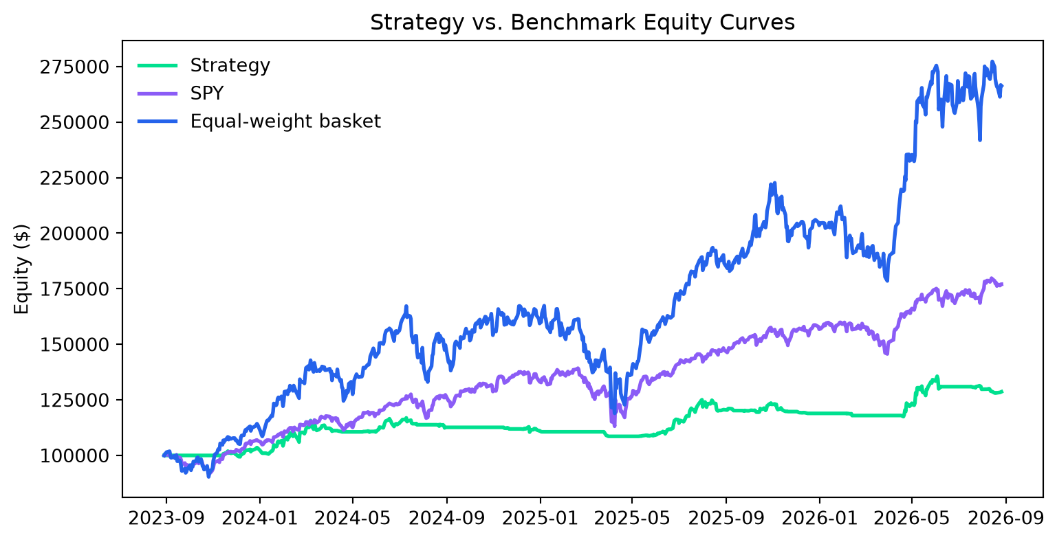
                     Final Equity  Total Return %
Strategy                 128657.0           28.66
SPY                      177038.0           77.04
Equal-weight basket 266324.0 166.32dd = (equity / equity.cummax() - 1) * 100
fig, ax = plt.subplots(figsize=(9, 3.5))
ax.fill_between(dd.index, dd.values, 0, color="#FF4D6A", alpha=0.35); ax.plot(dd.index, dd.values, color="#FF4D6A", lw=1.2)
ax.set_ylabel("Drawdown (%)"); ax.set_title("Strategy Drawdown")
plt.show()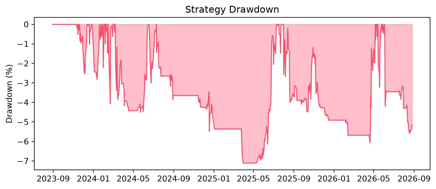
Mark-to-market share of equity held in positions.
exposure_pct = 100 * portfolio.asset_value(group_by=True) / equity
fig, ax = plt.subplots(figsize=(9, 3.5))
ax.plot(exposure_pct.index, exposure_pct.values, color="#2563EB", lw=1.4)
ax.set_ylabel("% of Equity Invested"); ax.set_title("Portfolio Exposure Over Time")
plt.show()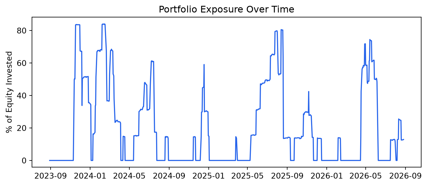
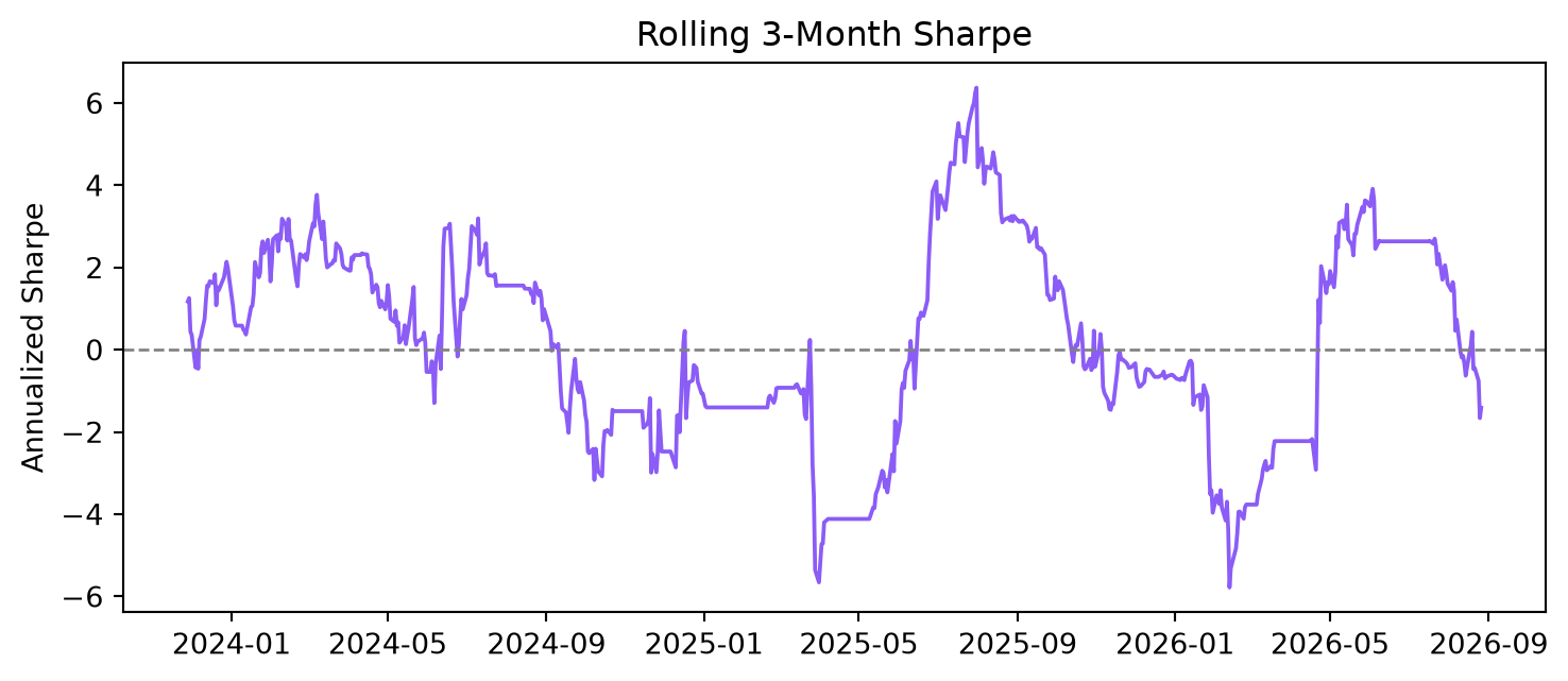
roll = returns.rolling(63).apply(lambda r: r.mean() / r.std() * np.sqrt(252), raw=True)
fig, ax = plt.subplots(figsize=(9, 3.5))
ax.plot(roll.index, roll.values, color="#8B5CF6", lw=1.4); ax.axhline(0, color="gray", ls="--", lw=1)
ax.set_ylabel("Annualized Sharpe"); ax.set_title("Rolling 3-Month Sharpe")
plt.show()