Code
library(blotter)
library(quantstrat)
library(TTR)
Sys.setenv(TZ = "UTC")
FinancialInstrument::currency("USD")R / quantstrat Research Notebook
Get the code: Download Strategy Code (.R) | Download Analysis Code (.R)
This notebook is a complete, executable replication of the strategy published at quantstr.at. Every number, table and chart below is produced by the R code in this document at render time; nothing is pasted in from the article. Re-running it (quarto render keltner-adx-volatility-breakout-qqq-R.qmd) reproduces every result from scratch against freshly downloaded market data.
The strategy, as specified:
Trade QQQ, NVDA, AAPL, MSFT, AMD, and AMZN using a Keltner Channel Volatility Breakout strategy. The channel is a 20-period EMA centre line with upper and lower bands set 2.0 x the 10-period ATR away from it. Enter long when the close breaks above the upper band and the 14-period ADX is above 25 (confirming trend strength). Exit when the close falls below the 20-period EMA centre line.
blotter is attached explicitly: quantstrat only lists it under Depends, and some sessions do not attach it, which breaks rm.strat()/initPortf().
library(blotter)
library(quantstrat)
library(TTR)
Sys.setenv(TZ = "UTC")
FinancialInstrument::currency("USD")Six large-cap U.S. technology names plus QQQ over a fixed three-year window. Each position is sized as one equal dollar slot (starting equity / number of symbols), so the portfolio is long-only and never levered.
symbols     <- c("QQQ", "NVDA", "AAPL", "MSFT", "AMD", "AMZN")
start_date  <- "2023-08-29"
end_date    <- "2026-08-27"
init_equity <- 100000

ema_n     <- 20    # Keltner centre line: EMA of the close
atr_n     <- 10    # Keltner band width: ATR period
atr_mult  <- 2     # Keltner band width: ATR multiplier
adx_n     <- 14    # trend-strength filter period
adx_min   <- 25    # entries require ADX above this level
slot_usd  <- init_equity / length(symbols)
cost_rate <- 0.0005  # 5 bps of traded value charged on every fill

stock(symbols, currency = "USD", multiplier = 1)Daily bars from Yahoo Finance. Yahoo’s close is already split-adjusted, so getSymbols(adjust = TRUE) would apply the split a second time (NVDA’s 10-for-1 split in June 2024 would show up as a 10x price jump). Instead the download is left raw and every OHLC column is scaled by Yahoo’s own Adjusted/Close ratio, which carries both splits and dividends once.
getSymbols(symbols, from = start_date, to = end_date, src = "yahoo", adjust = FALSE)[1] "QQQ" "NVDA" "AAPL" "MSFT" "AMD" "AMZN"for (sym in symbols) assign(sym, adjustOHLC(get(sym), use.Adjusted = TRUE))
# Data sanity check: no single-day move above 40% in any adjusted series.
for (sym in symbols) {
worst <- max(abs(dailyReturn(Cl(get(sym)))))
if (worst > 0.40) stop(sprintf("%s has a %.0f%% one-day move: likely an unadjusted split.", sym, worst * 100))
}portfolio.st <- "KeltnerADX"
account.st <- "KeltnerADX"
strategy.st <- "KeltnerADX"
suppressWarnings(try(rm.strat(portfolio.st), silent = TRUE))
suppressWarnings(try(rm.strat(account.st), silent = TRUE))
suppressWarnings(try(rm.strat(strategy.st), silent = TRUE))
initPortf(portfolio.st, symbols = symbols, initDate = start_date, currency = "USD")
initAcct(account.st, portfolios = portfolio.st, initDate = start_date, currency = "USD", initEq = init_equity)
initOrders(portfolio.st, initDate = start_date)
strategy(strategy.st, store = TRUE)The Keltner Channel is an EMA centre line with bands set a multiple of the Average True Range above and below it. ADX measures trend strength.
keltner_channel <- function(HLC, n_ema = 20, n_atr = 10, mult = 2) {
  mid <- EMA(Cl(HLC), n = n_ema)
  atr <- ATR(HLC, n = n_atr)[, "atr"]
  out <- cbind(mid - mult * atr, mid, mid + mult * atr)
  colnames(out) <- c("lower", "mid", "upper")
  out
}

add.indicator(strategy.st, name = "keltner_channel",
              arguments = list(HLC = quote(HLC(mktdata)), n_ema = ema_n, n_atr = atr_n, mult = atr_mult),
              label = "Keltner")
add.indicator(strategy.st, name = "ADX",
              arguments = list(HLC = quote(HLC(mktdata)), n = adx_n),
label = "ADX")Entry fires on the first bar where the close is above the upper band AND ADX is above its threshold. Exit fires when the close crosses below the EMA centre line.
add.signal(strategy.st, name = "sigComparison",
           arguments = list(columns = c("Close", "upper.Keltner"), relationship = "gt"), label = "above_upper")
add.signal(strategy.st, name = "sigThreshold",
           arguments = list(column = "ADX.ADX", threshold = adx_min, relationship = "gt"), label = "adx_strong")
add.signal(strategy.st, name = "sigFormula",
           arguments = list(formula = "above_upper & adx_strong", cross = TRUE), label = "entry")
add.signal(strategy.st, name = "sigCrossover",
arguments = list(columns = c("Close", "mid.Keltner"), relationship = "lt"), label = "exit")Orders fill at the next bar’s open (prefer = "Open"), so a signal can only be acted on after the bar that produced it has closed. Every fill pays 5 bps of traded value.
fill_cost <- function(TxnQty, TxnPrice, Symbol) -abs(TxnQty * TxnPrice) * cost_rate

# Position sizing: whole shares worth one equal dollar slot at the signal bar's
# close, and nothing while the symbol is already held (no pyramiding).
osEqualSlot <- function(data, timestamp, orderqty, ordertype, orderside, portfolio, symbol, ruletype, ..., slot) {
  if (getPosQty(portfolio, symbol, timestamp) > 0) return(0)
  floor(slot / as.numeric(Cl(data[timestamp])))
}

add.rule(strategy.st, name = "ruleSignal",
         arguments = list(sigcol = "entry", sigval = TRUE, orderqty = 1, ordertype = "market",
                          orderside = "long", osFUN = "osEqualSlot", slot = slot_usd,
                          replace = FALSE, prefer = "Open", TxnFee = "fill_cost"),
         type = "enter", label = "EnterLong")

add.rule(strategy.st, name = "ruleSignal",
         arguments = list(sigcol = "exit", sigval = TRUE, orderqty = "all", ordertype = "market",
                          orderside = "long", replace = TRUE, prefer = "Open", TxnFee = "fill_cost"),
type = "exit", label = "ExitLong")applyStrategy(strategy.st, portfolio.st)
updatePortf(portfolio.st)
updateAcct(account.st)
updateEndEq(account.st)One row per symbol: closed-trade count, net P&L, win rate and profit factor.
tstats <- tradeStats(portfolio.st)
print(tstats[, c("Symbol", "Num.Trades", "Net.Trading.PL", "Percent.Positive", "Profit.Factor", "Max.Drawdown")])
Symbol Num.Trades Net.Trading.PL Percent.Positive Profit.Factor
AAPL AAPL 10 -741.648 40.00000 0.8288993
AMD AMD 8 17794.526 75.00000 6.6680062
AMZN AMZN 9 -4083.069 22.22222 0.2143304
MSFT MSFT 6 1706.182 50.00000 2.5797711
NVDA NVDA 7 11960.370 42.85714 4.9150907
QQQ QQQ 8 2603.131 62.50000 3.4627244
Max.Drawdown
AAPL -5072.780
AMD -5810.985
AMZN -5006.190
MSFT -1735.425
NVDA -3562.570
QQQ -1359.987This section continues in the same R session, reusing the portfolio, account and price data built above.
library(PerformanceAnalytics)
strategy_eq <- getAccount(account.st)$summary$End.Eq
final_eq <- as.numeric(last(strategy_eq))
total_ret_pct <- (final_eq / init_equity - 1) * 100
strategy_ret <- dailyReturn(strategy_eq)
ann_ret_pct <- as.numeric(Return.annualized(strategy_ret)) * 100
sharpe <- as.numeric(SharpeRatio.annualized(strategy_ret, Rf = 0))
maxdd_pct <- as.numeric(maxDrawdown(strategy_ret)) * 100
tstats_kpi <- tradeStats(portfolio.st)
n_trades <- sum(tstats_kpi$Num.Trades)
n_winners <- sum(round(tstats_kpi$Percent.Positive / 100 * tstats_kpi$Num.Trades))
win_rate <- n_winners / n_trades * 100
profit_factor <- sum(tstats_kpi$Gross.Profits) / abs(sum(tstats_kpi$Gross.Losses))
kpi_df <- data.frame(
  Metric = c("Final Equity", "Total Return", "Annualized Return", "Annualized Sharpe",
             "Max Drawdown", "Closed Trades", "Win Rate", "Profit Factor"),
  Value = c(sprintf("$%s", format(round(final_eq), big.mark = ",", scientific = FALSE)),
            sprintf("%.2f%%", total_ret_pct), sprintf("%.2f%%", ann_ret_pct), sprintf("%.2f", sharpe),
            sprintf("%.2f%%", maxdd_pct), sprintf("%d", n_trades), sprintf("%.1f%%", win_rate),
            sprintf("%.2f", profit_factor)))
gt::gt(kpi_df) |>
  gt::tab_header(title = "Headline Results", subtitle = sprintf("%s to %s", start_date, end_date)) |>
gt::cols_align(align = "right", columns = "Value")| Headline Results | |
| 2023-08-29 to 2026-08-27 | |
| Metric | Value |
|---|---|
| Final Equity | $129,239 |
| Total Return | 29.24% |
| Annualized Return | 8.99% |
| Annualized Sharpe | 1.02 |
| Max Drawdown | 6.99% |
| Closed Trades | 48 |
| Win Rate | 47.9% |
| Profit Factor | 2.71 |
The strategy against two passive benchmarks over the same window: SPY buy-and-hold and an equal-weight buy-and-hold basket of the traded symbols.
spy <- getSymbols("SPY", from = start_date, to = end_date, auto.assign = FALSE, src = "yahoo", adjust = FALSE)
spy <- adjustOHLC(spy, use.Adjusted = TRUE)
spy_eq <- init_equity * Cl(spy) / as.numeric(Cl(spy)[1])
basket_eq <- Reduce(`+`, lapply(symbols, function(s) {
  px <- Cl(get(s)); (init_equity / length(symbols)) * px / as.numeric(px[1])
}))
comparison <- merge(strategy_eq, spy_eq, basket_eq, join = "inner")
colnames(comparison) <- c("Strategy", "SPY", "Equal-weight basket")
plot(as.zoo(comparison), plot.type = "single", col = c("#00E08F", "#8B5CF6", "#2563EB"),
     lwd = 2, xlab = "", ylab = "Equity ($)", main = "Strategy vs. Benchmark Equity Curves")
legend("topleft", legend = colnames(comparison), col = c("#00E08F", "#8B5CF6", "#2563EB"), lwd = 2, bty = "n")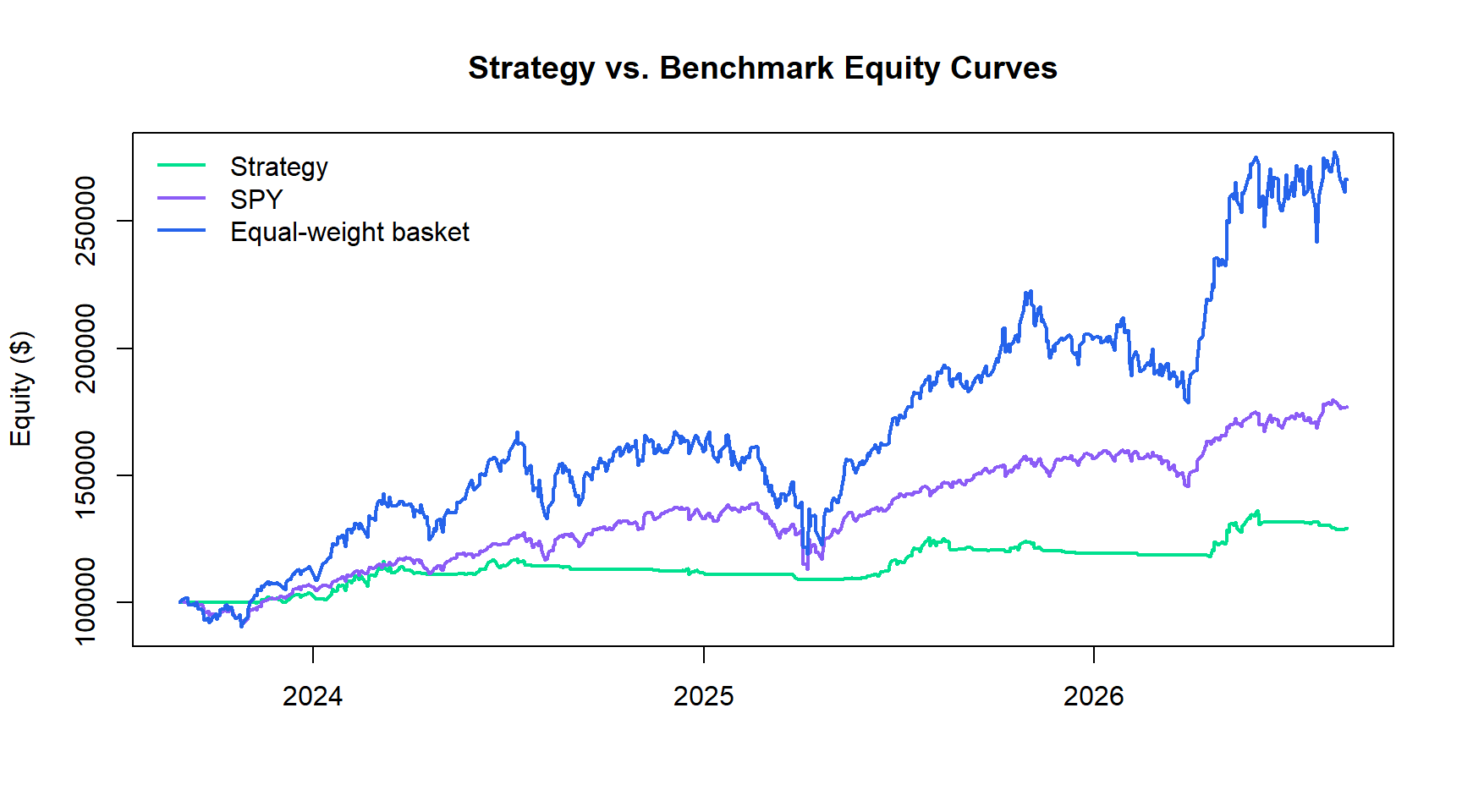
bench_final <- as.numeric(last(comparison))
gt::gt(data.frame(Series = colnames(comparison),
                  `Final Equity` = sprintf("$%s", format(round(bench_final), big.mark = ",")),
`Total Return` = sprintf("%.2f%%", (bench_final / init_equity - 1) * 100), check.names = FALSE))| Series | Final Equity | Total Return |
|---|---|---|
| Strategy | $129,239 | 29.24% |
| SPY | $177,038 | 77.04% |
| Equal-weight basket | $266,324 | 166.32% |
dd <- Drawdowns(strategy_ret) * 100
plot(as.zoo(dd), col = "#FF4D6A", lwd = 1.5, xlab = "", ylab = "Drawdown (%)", main = "Strategy Drawdown")
abline(h = 0, lty = 2, col = "gray60")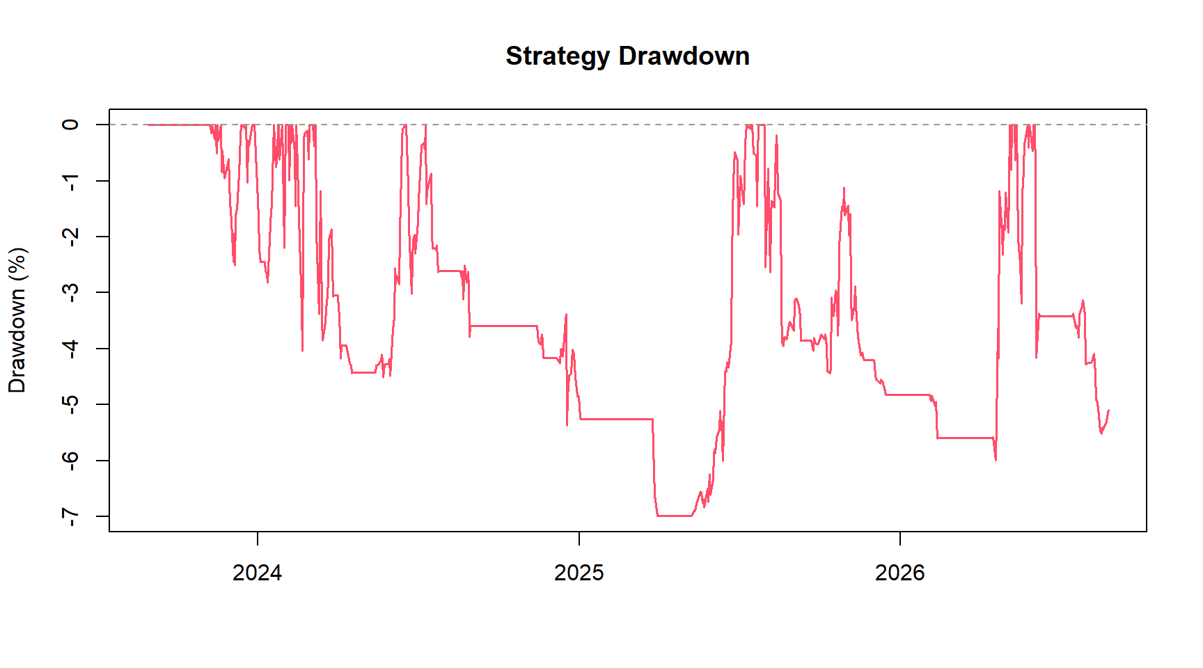
Mark-to-market share of equity held in positions, from blotter’s own position values.
pos_value <- Reduce(`+`, lapply(symbols, function(s) getPortfolio(portfolio.st)$symbols[[s]]$posPL.USD$Pos.Value))
exposure_pct <- 100 * merge(pos_value, strategy_eq, join = "inner")[, 1] / merge(pos_value, strategy_eq, join = "inner")[, 2]
plot(as.zoo(exposure_pct), col = "#2563EB", lwd = 1.5, xlab = "", ylab = "% of Equity Invested", main = "Portfolio Exposure Over Time")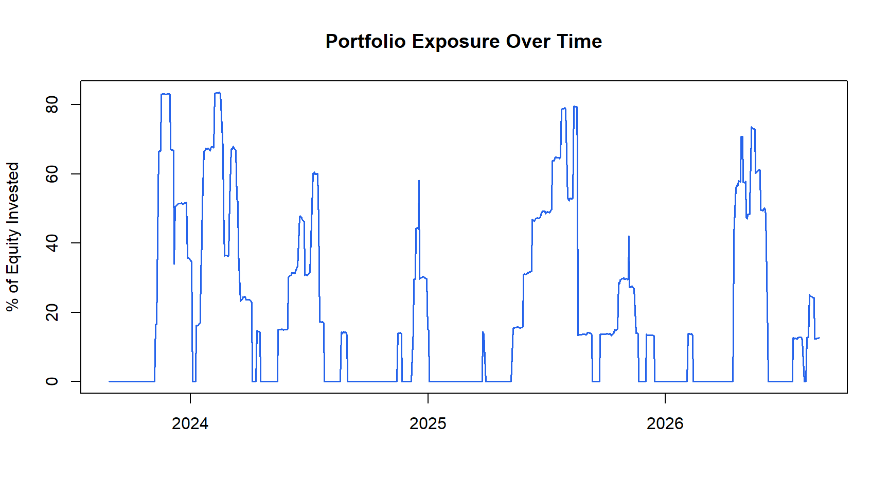
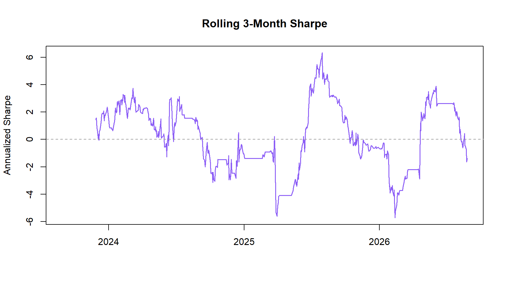
roll <- rollapply(strategy_ret, width = 63, FUN = function(r) mean(r) / sd(r) * sqrt(252), align = "right", fill = NA)
plot(as.zoo(roll), col = "#8B5CF6", lwd = 1.5, xlab = "", ylab = "Annualized Sharpe", main = "Rolling 3-Month Sharpe")
abline(h = 0, lty = 2, col = "gray60")